Modelling Primary and Secondary Pump Loops in TPD

We will often have to edit the water-side systems created by the wizard. One common reason is to replace a basic setup with a system which has a primary pump loop for the plant equipment, and one or more secondary pump loops distributing water around the building.

Before attempting the setups shown in this guide, you should be familiar with the topic of splitting and recombining plant flows, covered here.

Let’s begin by taking one of the setups from the previous blog post; there are three heating collections and two boilers in parallel.

The flow rates are specified rather than sized, and the correct splitting of flows is ensured by the design flow rate entered into the valves.

There is a single pump which is controlled to run when any of the collections has a load.

For this starting case, we are not using variable flow capacity on the heating collections.

We can very quickly turn this into a primary-secondary setup by replacing the valves with pumps, and adding another pipe (highlighted).

Note that the secondary pumps are connected to the controller of their respective collection. Now each secondary pump will run when its respective collection has a load. The primary pump will run whenever any collection has a load (note the MAX controller).

On hours when only one or two collections have a load, any excess flow from the primary pump will be recirculated in the primary loop.

On hours when all the collections have a load, there is no excess flow to recirculate; all of the flow from the primary pump is sent to a collection.

Note that it is possible for the sum of the secondary pump flow rates to exceed the flow rate of the primary pump; to some extent the rules established in the previous blog post do not apply for primary-secondary setups. This is potential pitfall, however, as there is no error message to warn us that the flow rates are unbalanced and we may have water flowing in an unwanted direction, leading to unwanted temperatures. In this image the flow rate of every pump is 0.9 l/s and the water temperature supplied to the collections has fallen below the target of 71 C.

If we return the pump flow rates to the correct values and delete the wires connecting the secondary pumps to their controllers, we can use the variable flow capacity option on the collections.

Let’s change how the boilers are used now. Let’s only use both boilers if the required heating load is over 50% of the maximum value.

There are a few ways we could detect this switching point; for the sake of this example we are going to test the return water temperature in the primary loop.

We have a setpoint of 71 C and a delta T of 11 C, so for a 50% load we might expect a return temperature of about 65.5 C. Let’s put a controller on the valve of one of the boilers and switch the control signal around this temperature.

We can soon see the impact on the results, compared to the case where the flow is always split evenly between the boilers.

Of course, we could just use a multiboiler component to achieve a similar result instead of two separately controlled boilers. But there may be instances where we prefer to model two separate boilers in this fashion, for example to use a wide control band as in the example above, or in a case where there are further components which we need to take into account (if, for example, one of the boilers was preceded by an exchanger to a different plant loop). There may also be a difference in pump load which needs to be taken into account; on that note, if the boilers and valves are replaced by a multiboiler we should ensure that its pressure drop matches the sum of the pressure drops of the components we have replaced (e.g. 25 kPa for the valve and 25 kPa for the boiler becomes 50 kPa for the multiboiler).

We can try to simplify the setup further; as we are using variable flow capacity on the collections we could experiment with replacing these three collections with a single one and allow the varying flow capacity to provide the flow we need (assuming we don’t need to see the heating load split between the three collections in our results). In this example the difference made to pumping power was around 0.1%, so no major error was introduced; in fact, as simpler systems generally simulate more smoothly and with fewer simulation events, in most situations we are more likely to remove a source of error by simplifying the model.

It’s not necessary with such a simple example, but it can sometimes be expedient to separate loops with a 100% efficient exchanger. This is a convenient way to stop pressure and flows from one loop affecting what’s happening in a connected loop, while still conveying 100% of the heat energy as if the water flows were uninterrupted. This is a particularly useful strategy in cases where pressure-related errors are occurring, or errors relating to negative flow through components.

Using this exchanger technique we can make a variation on an earlier setup; two boilers,
this time in series rather than parallel, with the second controlled only to be used for loads over 50% of the peak.

The first boiler in the loop is controlled to be used whenever there is a load at the collection (or rather, its pump is controlled like this, but remember the boiler will only run whenever there is flow through it).

The second boiler is controlled to be used when the water temperature leaving the first boiler is below the setpoint of 71 C, but only on hours when there is a load (note the MIN controller).

If each boiler is sized for 50% of the total load, and the exchanger efficiency is 100%, then this setup will work just fine. This could be a useful setup if we had a pump associated with each boiler and wanted to see this fact reflected in the results.

We can take this latest example and change it into a very simple-looking setup.

We have used the ancillary load property to remove the boiler pumps from the schematic and, in effect, absorb them into the multiboiler component.

We set the profile modifiers so that ancillary load 1 is used when the heating load is positive, and ancillary load 2 is used when the heating load is over 50%.

If the collection is using variable flow capacity then we don’t even require a controller for the pump.

It is often better to use an elegant solution that gives the correct results, rather than create a complicated setup which matches a schematic drawing. Whether simplification is suitable will depend on the information available and the results detail required, but there are normally several ways to reach similar or even identical results.

Splitting TPD Plant Room Flows

We will often want to create plant room layouts which are more complex than the ones created by the systems wizard, and split and combine flows to use components on separate branching pipes. There are different ways to achieve this, but also a few potential pitfalls; this guide aims to shed some light on the subject.

In the image above we have used the wizard to create three heating circuits because we wish to view the results for each collection separately. But what if we want to have the three heating collections on the same heating loop, served by the same heating source? We might decide wouldn’t be appropriate to put the collections in series as the water temperatures into the second and third collections would be too low. 

In order to put the collections in parallel we will need to use junctions to split and combine the water flow.

Each collection has a controller checking to see if the load is above zero, and the pump has a “max” controller so that it will run if any signal is greater than zero.

If we’re not careful, however, soon we could start running into problems. Here is one message we might well encounter.

Why has this happened?
Why do we have an inconsistent design flow rate?
Let’s look at the parameters which will affect flow sizing:

If we calculated the sized flow rates for the boiler and collections from their maximum loads and delta T, for this model we would find:

Boiler: 0.68 l/s
Heating A: 0.16 l/s
Heating B: 0.32 l/s
Heating C: 0.41 l/s

The 0.68 l/s of the boiler does not match the 0.89 l/s total required by the heating collections. This is the inconsistency referred to in the error message. In other words,

0.16 + 0.32 + 0.41 =/= 0.68.

How can it be fixed? We can either balance the equation or we can remove the boiler from the flow sizing altogether. If we set the boiler delta T to “none” then it won’t be used in the pump sizing and it will just accept whatever flow is required by the collections. Alternatively, we could, for example, change the delta T to 11 for the collections currently using 8; when the components have the same sizing parameters the equation will balance:

0.16 l/s + 0.23 l/s + 0.29 l/s = 0.68 l/s

This setup will still work if we want to incorporate varying flow rates; we can assign variable flow capacity to the collections and the flow rate will decrease for lower heating loads.

When we’re using the variable flow capacity on all the collections there is no more need for the controllers on the pump; the collections’ capacity will increase or decrease to allow the hot water to flow as and when it is needed, and only where it is needed, for example on this hour when only collection C has a heating load:

If we wanted to, we could take our earlier example and replace the multi-boiler with two boiler components, each with a sizing factor of 0.5, and put them in parallel; as long as the boilers are sized using the same delta T the pump sizing will succeed.

What if we didn’t want to size these flows, and instead we wanted to dictate the pump maximum flow rate and the maximum flow rate which will travel down each pipe? Let’s enter a set value for the pump flow rate and add some valves to the system.

Now we might run into an inconsistent design flow rate issue again. The error says that it might relate to the collection “Heating C”, but we shouldn’t take this too literally; this tells us that the heating system has the problem but we will have to check the whole system.

Let’s look at the design flow rate values we’ve entered into our components…

The total flow rate for the valves associated with the collections is 0.3 + 0.3 + 0.3 = 0.9, the same as the pump flow rate. So the problem probably isn’t related to the heating collections after all.

Let’s check the boilers: 0.75 + 0.75 = 1.5 l/s, which is inconsistent with the 0.9 l/s pump flow rate.

Consider what would happen where the boiler flows join before entering the pump; how could 1.5 l/s become 0.9 l/s? It cannot, so the simulation fails. On the other hand, on the other side of the pump there is no problem splitting 0.9 l/s into 0.3 + 0.3 + 0.3.

0.9 = 0.3 + 0.3 + 0.3
0.9 =/= 0.75 + 0.75

We could fix this easily by changing the boiler valve flow rates to 0.45 l/s each.

0.9 = 0.3 + 0.3 + 0.3
0.9 = 0.45 + 0.45

What if we encounter a message about an error calculating capacities?

We’ve already ensured that the flow rates are inconsistent. We now need to check either the component capacities, or pressure drops (note that only one or the other of these parameters will be specified at any time for a given component).

In this system we have specified a pressure drop for each component (and for the pump, a peak pressure value). As before, we should check the whole circuit and not just the component mentioned in the message.

Whereas with the flow rates we needed to ensure that the total flow rates on either side of a junction are equal (e.g., 0.45 and 0.45 combining into 0.9), with the pressure drops we instead need to ensure that when flows split and join the pressure drops on the branching pipes are equal to one another. Let’s break this down further:

Here we have two branches. The flow returning from the heating collections (yellow pipe) reaches a junction and is split between the two boilers. Their flows then recombine and enter the red pipe.

The pressure drop on the top branch is 25 + 50 = 75 kPa. The pressure drop on the bottom branch is 25 + 25 = 50 kPa. 50 and 75 are not equal, so we need to edit the components to balance the equation (e.g., by changing the pressure drop of the top-most valve to 25 kPa).

Meanwhile for the collections the flow from the pump (red) is split into three branches which recombine (yellow).

From top to bottom, the total pressure drop of the branches is:

25 + 25 = 50 kPa
25 + 25 = 50 kPa
50 + 25 = 75 kPa

50 and 75 are not equal. Again, we can change the pressure drop of the bottom-most valve to 25 kPa to remedy this.

We would also receive an error message like this if the peak pressure of the pump was insufficient.

In this example, if every valve, boiler, and collection had a pressure drop of 25 kPa, we could draw the diagram below:

On a complete circuit the water loses 100 kPa of pressure and the pump has to overcome this; the pump peak pressure must be 100 kPa or more.

Now the design flow rates and pressure drops are in balance, and the pump is strong enough to move the water.

The schematic is rather messy. Is there a more elegant solution?

As the error messages above have hinted, the point of the design flow rates and design pressure drops is to get a flow “capacity” value for the components. You can choose to just type this in directly.

Note that this value is not really appropriate for this component, but it is convenient; more on this later.

This approach makes it very easy to split flows equally between branching pipes.

The valves have all been deleted and a capacity of 1 has been entered into each boiler and collection.

Note that we can now adjust the ratio of flow rates between branches very easily; for example, if the capacity of the boilers is in the ratio 5:1 then the flows will take on the same ratio.

Note that this approach of using capacities will also work if we wanted to size the pump flow rate rather than specify it, as long as we set a delta T value to our collections and/or boilers.

One major downside of using capacities like this is it can be hard to get the correct pump load, which is related closely to pressure drop. By using such large capacity values, we have a negligible pressure drop and pump load. We can work around this by adding a valve in series with the pump which has a pressure drop representing the drop around the whole system, and whose flow is sized in the same way as the pump, either “Auto” (sized) or a fixed value:

As before, if it is appropriate for our design, we can turn on the variable capacity option for the collections and do away with the controllers.

In the next blog post on this topic we will look at modelling primary and secondary loops.

Drawing Dormer Windows

Windows which project from a pitched roof can be drawn without difficulty in the Tas 3D modeller. This short guide shows how to achieve this on five example models, using a methodical approach and knowledge of the “intersect planes” tool.

It is recommended that users should be familiar with different techniques for drawing roofs before following this guide. See here for more details.

Example 1

This is the easiest example, a flat-roofed wall dormer. The face of the dormer is coplanar with the external wall and there is no roof void to worry about.

Firstly, create the planes which will define the pitched roof. (On the “drawing utilities” tab, under “3D planes”, use the tool “by points”). Do not apply any planes at this stage.

Now create a plane where all points are equal to the height of the flat roof over the dormer. The reason will become clear in the next step.

Select the space. On the “drawing utilities” tab, under “3D planes”, find the tool “intersect planes”. Select the pitched roof plane and the horizontal plane which you have just created.

This will create a null wall across the space where the pitched roof and flat roof will intersect. From this line, draw null walls to the external wall (on a real project, refer to your drawings for the dormer side wall positions).

Place the window.

Recommended but optional: Clean up null lines.

Now apply the 3D planes. Note that for the flat roof over the dormer you can either use the horizontal plane created earlier or just enter a value for the space height.

Apply zones. Create the 3D analysis model.

In the list of building elements, change the null-exposed element to represent an external wall. Be sure to assign an appropriate construction to this building element in the TBD.

Finished!

In the following examples you can see how these techniques can be used to model window types that could seem challenging at first glance.

Example 2

Here we have a gable-fronted wall dormer. The face of the dormer is coplanar with the external wall and there is no roof void to worry about. But we do have to deal with two pitched roofs over the dormer – this is not a major obstacle as long as we remember how to use the intersect planes tool.

As in the previous example, begin by creating the planes which will define the main pitched roof.

Draw null lines marking the middle and limits of the dormer (on a real project, follow your drawings).

Create the planes which will define the pitched roof over the dormer. Note that it doesn’t matter if the points selected are not within the limits of the dormer’s location according to your drawings – as long as the points are on the correct line, the planes will intersect correctly with the main roof plane to define the dormer limits.

Select one of these spaces and intersect the corresponding dormer roof plane and the main roof plane. Do the same for the other space.

Place the window. Clean up null lines. Apply 3D planes.

Apply zones. Create the 3D analysis model. In the list of building elements, change the null-exposed element to represent an external wall.

Finished!

Example 3

This is similar to example 2 but we have the added complication of a roof void in some parts of the space. Thankfully, the use of 3D planes means the voids will not make our task any more difficult.

Firstly, create the planes which will define the main pitched roof. Draw null lines marking the middle and limits of the dormer (on a real project, follow your drawings).

Create the planes which will define the pitched roof over the dormer.

Select one of these spaces and intersect the corresponding dormer roof plane and the main roof plane. Do the same for the other space.

Draw the internal walls which separate the occupied space and the roof void (on a real project, follow your drawings). Also change the sides of the dormer to internal walls so that a solid wall separates the occupied space from the roof void.

Place the window. Clean up null lines. Apply 3D planes. Note that you can select multiple spaces and assign the same plane to them at the same time.

Apply zones. Create the 3D analysis model.

In the list of building elements, change the internal wall-exposed element (and if necessary, null-exposed element) to represent an external wall. Be sure to assign an appropriate construction to this building element in the TBD.

Finished!

Example 4

By now you can probably see how these techniques can be easily applied to a situation where a dormer window is set back from the external wall. Here we have another gable-roofed dormer and roof void situation, but the window is not coplanar with the external wall.

Firstly, create the planes which will define the main pitched roof. Draw null lines marking the middle and side limits of the dormer (on a real project, follow your drawings).

Create the planes which will define the pitched roof over the dormer. Note that it doesn’t matter if the points selected are not within the limits of the dormer’s location according to the plans – as long as the points are on the correct line, the planes will intersect correctly to define the dormer limits.

Select one of these spaces and intersect the corresponding dormer roof plane and the main roof plane. Do the same for the other space.

Draw the internal walls which separate the occupied space and the roof void (on a real project, follow your drawings). Change the sides of the dormer to internal walls. Draw an internal wall (not external) at the face of the dormer (on a real project, follow your drawings).

Place the window. Clean up null lines. Apply 3D planes.

Apply zones. Create the 3D analysis model. In the list of building elements, change the internal wall-exposed element (and if necessary, null-exposed element) to represent an external wall.

Finished!

Note how the different treatment of “internal wall” and “internal wall-exposed” allows us to have one building element separating the occupied space from the void space, and a different building element separating the occupied space from the outside air.

Example 5

Here we have a hip roof dormer set back from the wall, with a roof void. This is the most complicated example but by now you probably see clearly how to model it. Essentially this is the same as the previous example but with an additional step for the additional plane.

Firstly, create the planes which will define the main pitched roof. Draw null lines marking the middle and side limits of the dormer (on a real project, follow your drawings). Create the planes which will define the pitched roof over the dormer.

Draw an internal wall (not external) at the face of the dormer (on a real project, follow your drawings).

Draw a null line which intersects the dormer centre-line at the apex of the pitched roof over the front of your dormer (on a real project, follow your drawings).

Create the plane which will define the pitched roof over the front of the dormer.

Intersect planes twice. Intersect the front dormer plane with the first dormer side plane. Intersect the front dormer plane with the second dormer side plane.

Clean up null lines. This ensures nothing will interfere with intersecting the main roof plane and the dormer side planes.

Intersect the dormer side roof planes and the main roof planes.

Draw the internal walls which separate the occupied space and the roof void (on a real project, follow your drawings). Change the sides of the dormer to internal walls.

Place the window. Clean up null lines. Apply 3D planes.

Apply zones. Create the 3D analysis model. In the list of building elements, change the internal wall-exposed element (and if necessary, null-exposed element) to represent an external wall.

Finished!

Applying the techniques demonstrated in these examples will allow you to model any dormer window type you are likely to encounter.

Drawing Roofs

There are many options for drawing roofs in the Tas3D modeller. This short guide explains when each option may be the best choice and clears up some common questions.

Option 1: Set Wall Height
Pros: A very quick solution for simple sloped roofs with a level ridge.
Cons: Unsuitable for any other type of roof.

Option 2: Set Space Height
Pros: A very quick solution for stepped flat roofs.
Cons: Unsuitable for sloped roofs.

Option 3: Set Point Height (Select Join)
Pros: Allows quick modelling of curved roofs and intersecting slopes.
Cons: Can be time-consuming with roofs that cannot be triangulated easily. Not suitable when there is an abrupt change in roof level.

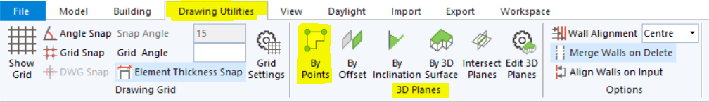
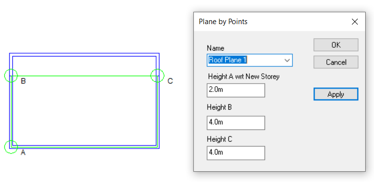
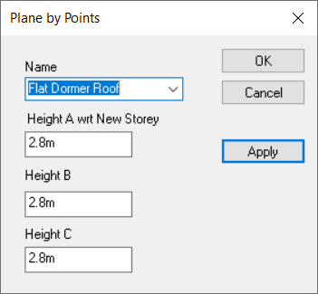
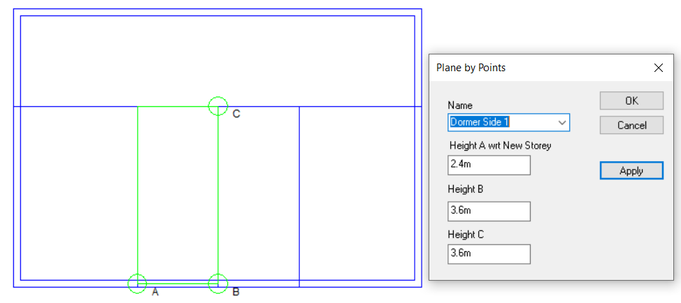
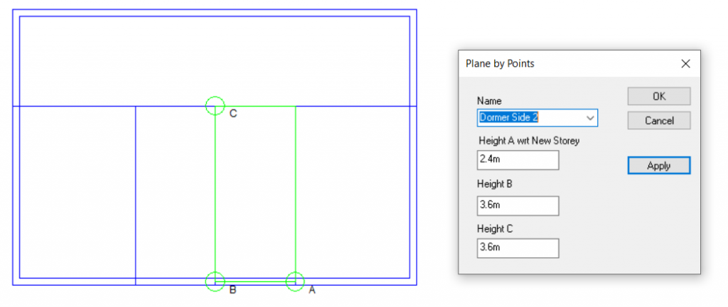
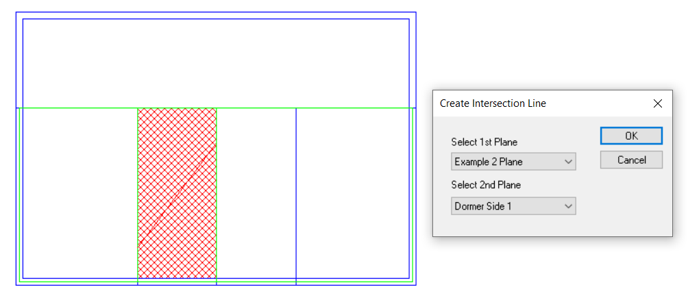
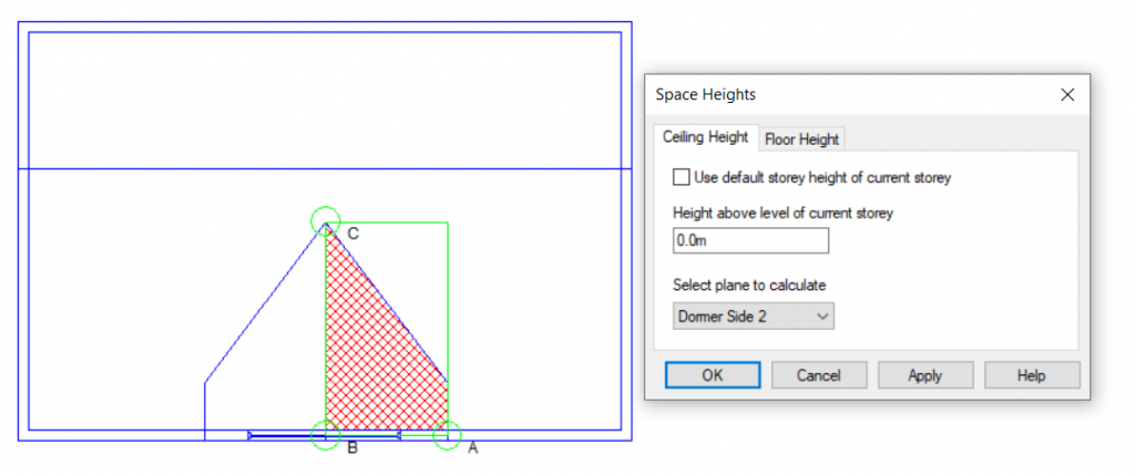
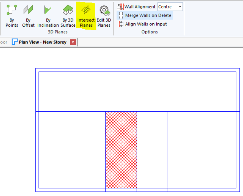
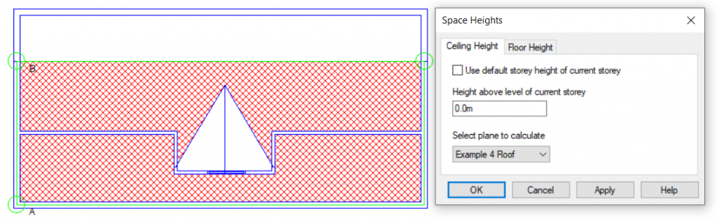
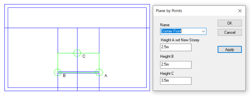
Option 4: Use 3D Planes
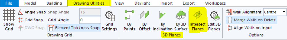
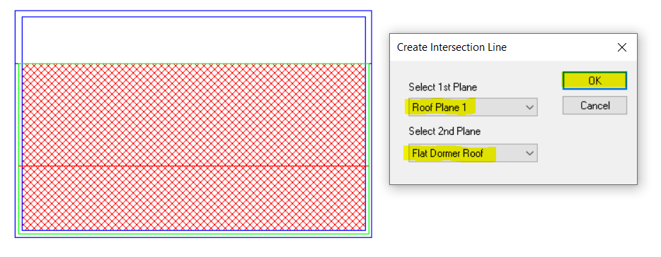
Pros: Can be applied to any sloping roof situation. Plane can be used for multiple roof areas at once. Intersection line between two planes can be calculated automatically. Reduces risk of errors arising from incorrect wall and point heights.
Cons: Creating the planes can be more time-consuming than the other methods.

Examples

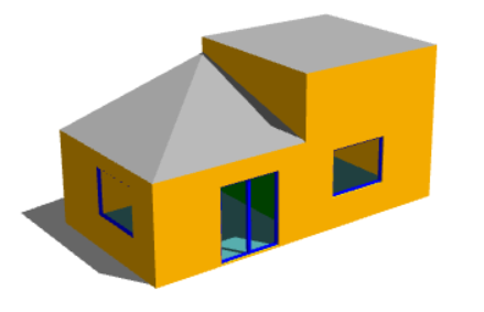
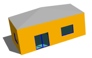
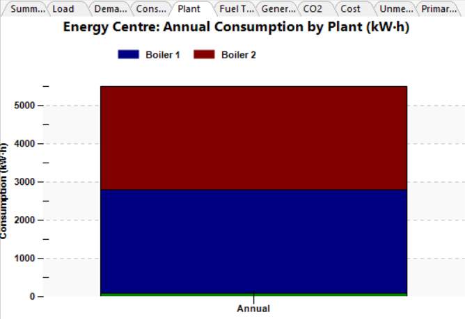
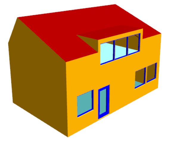
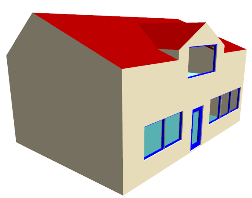
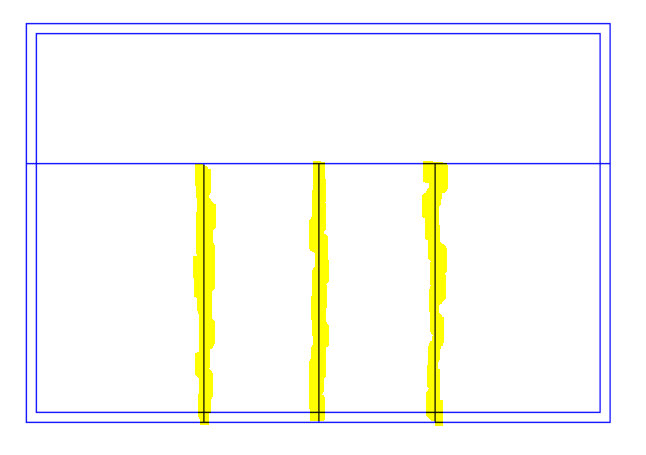
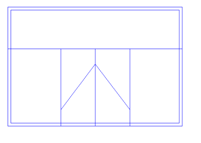
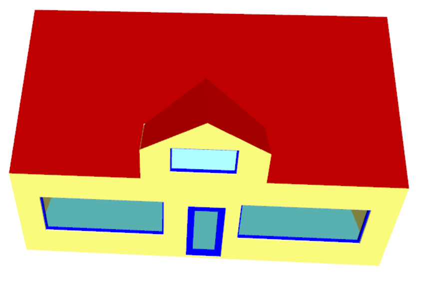
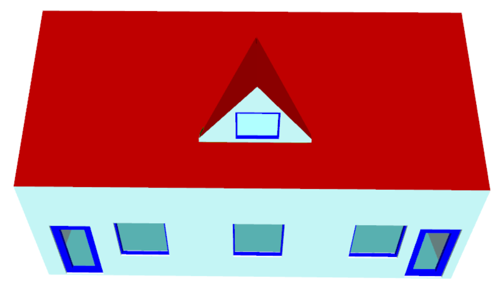
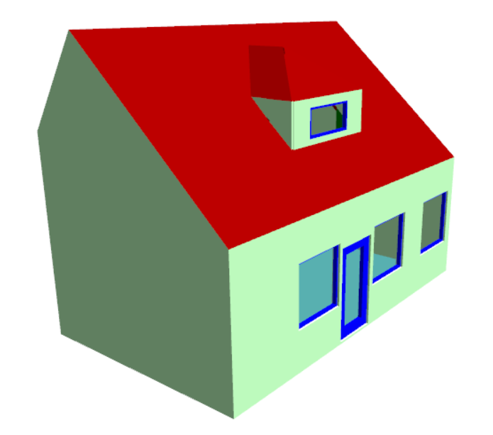
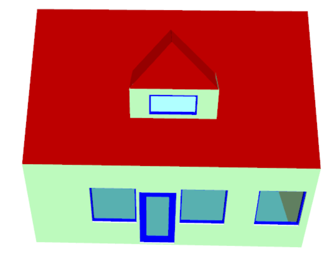
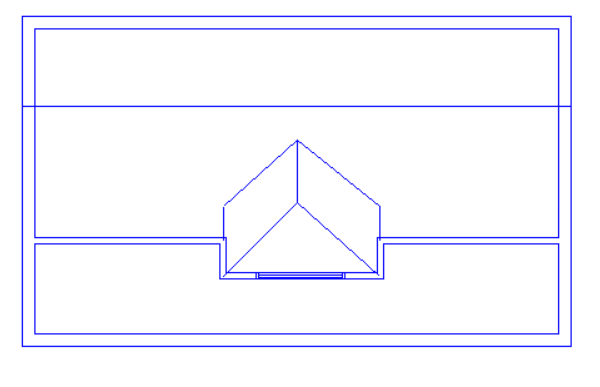
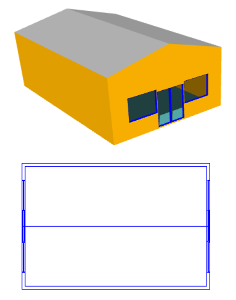
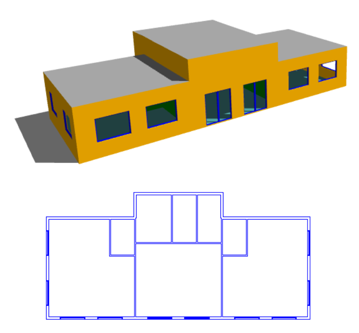
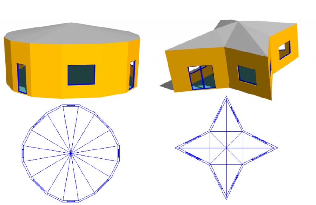
How would three different roofs be modelled most effectively on this simple building?

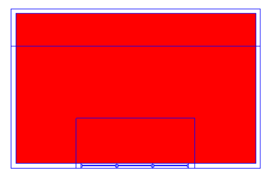
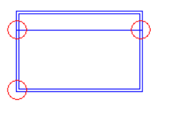
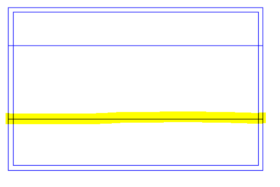
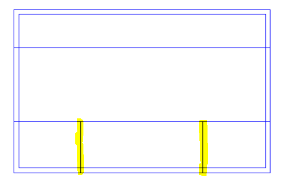
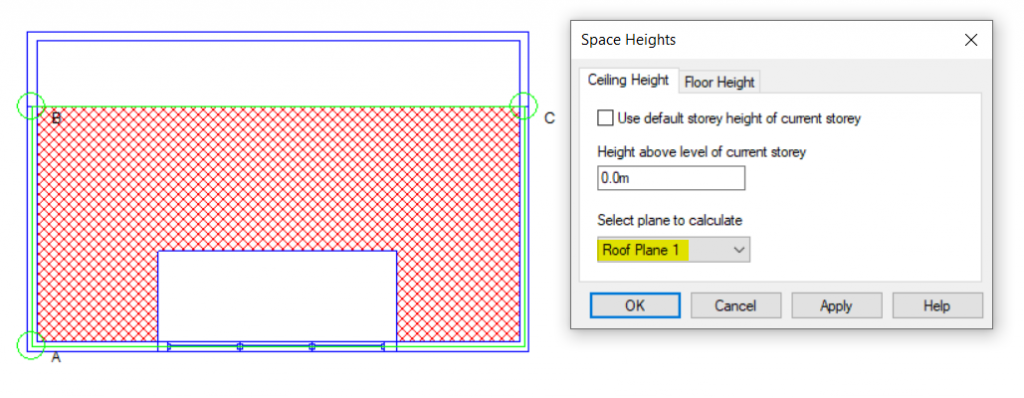
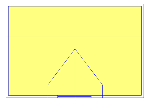
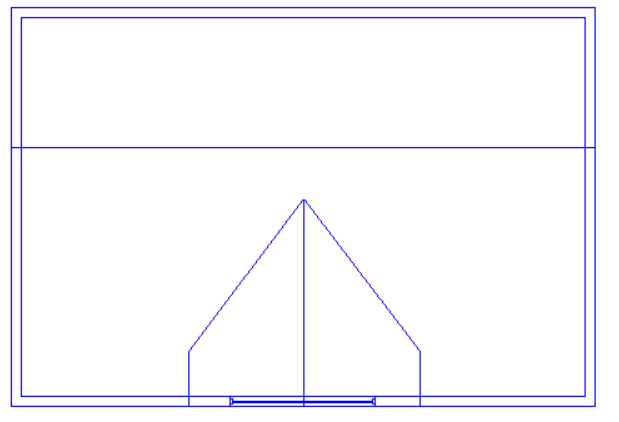
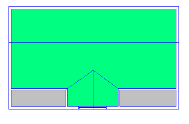
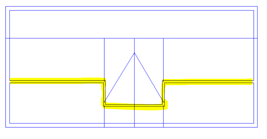
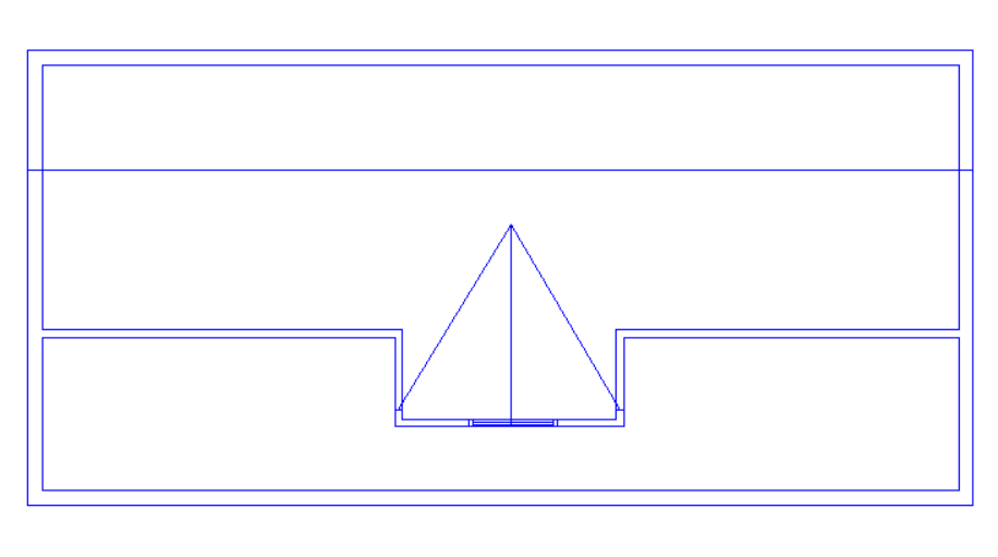
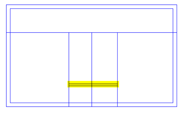
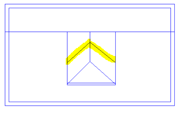
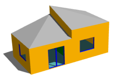
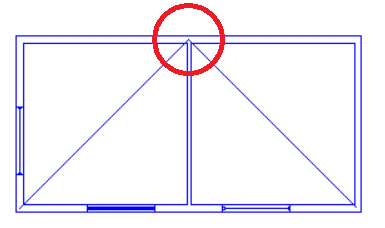
With this roof there is a sudden change in roof level, and the “Set Point Height” option cannot be used. We can see why if we consider one of the points used by both sloping roofs (highlighted in lower image) which would need to have two different roof heights at the same time; in this example it would need to be 4.5m for the left-hand roof and 5.5m for the right-hand roof.

We need to use 3D Planes here.

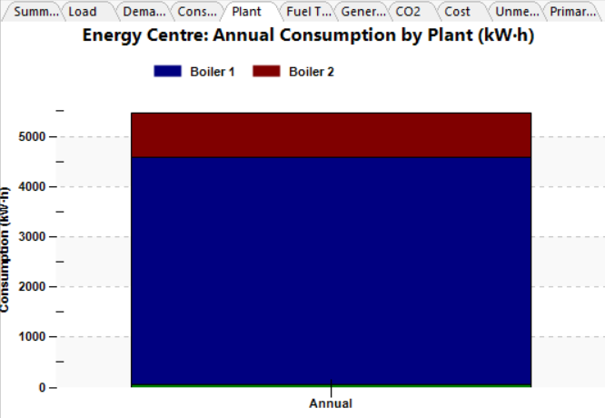
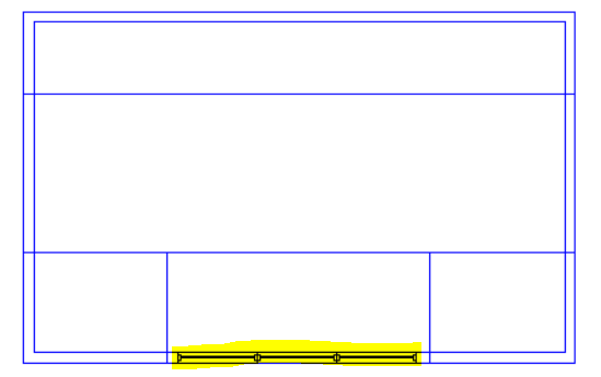
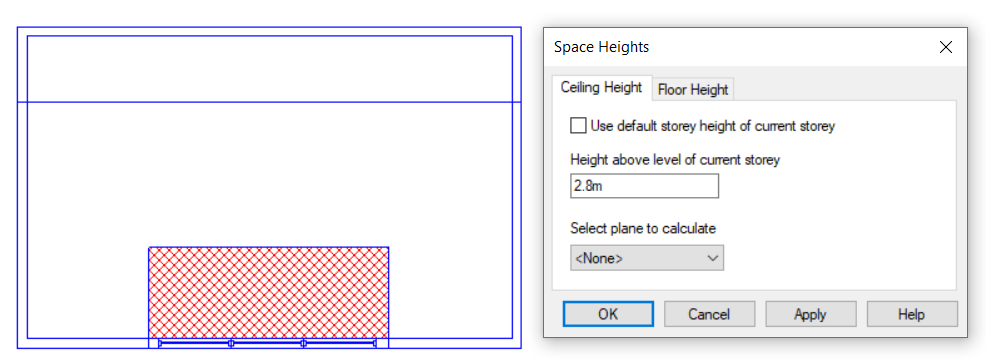
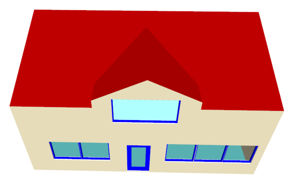
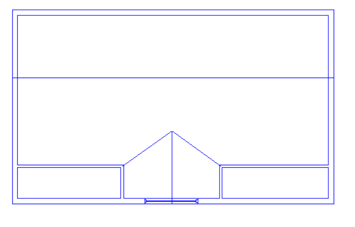
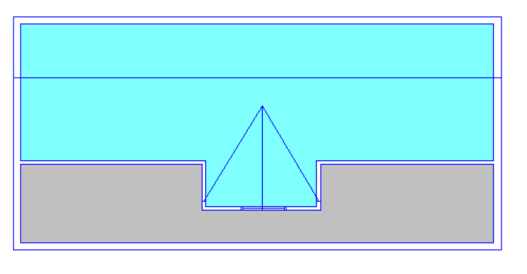
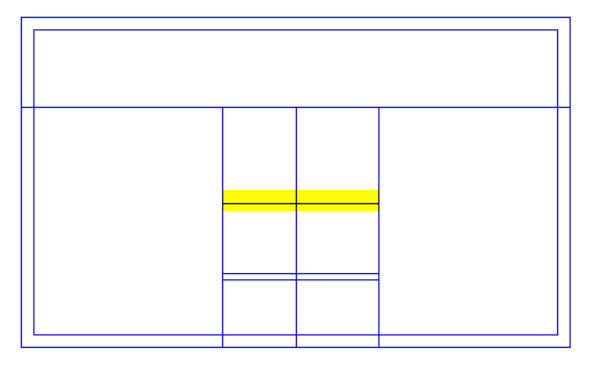
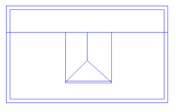
With this example we have a sudden change in roof level, meaning that once again we have points which would need to have two different heights at once; we cannot use the “Set Point Height” option.

In this case we would need to use 3D Planes for the left-hand roof. For the right-hand roof we can simply use the “Set Space Height” option.

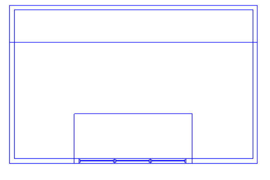
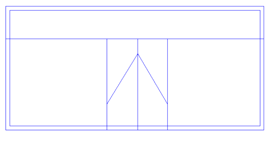
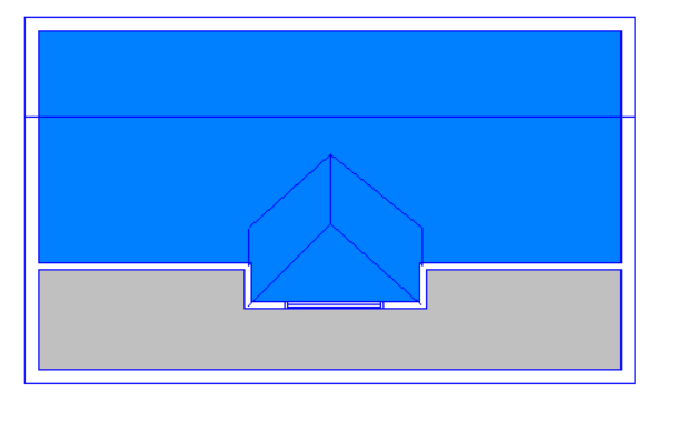
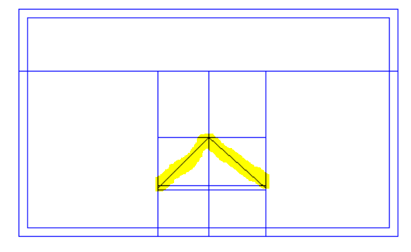
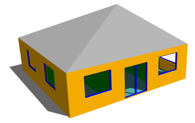
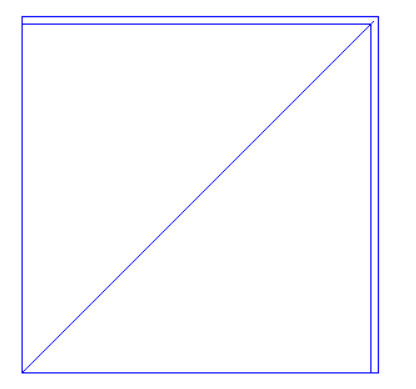
This roof rises to a single point and there is no step or sudden change in roof level. The roof can be achieved easily by using the “Set Point Height” option.

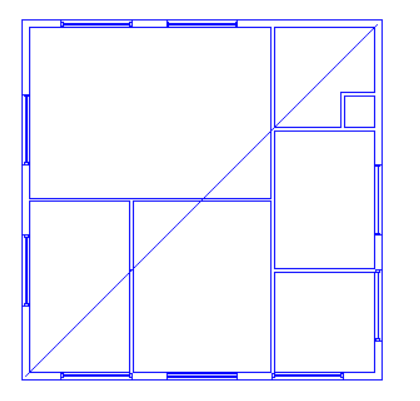
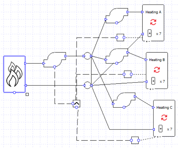
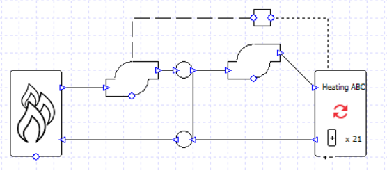
What about a situation where the roof itself is very simple, but there are several internal walls underneath it?

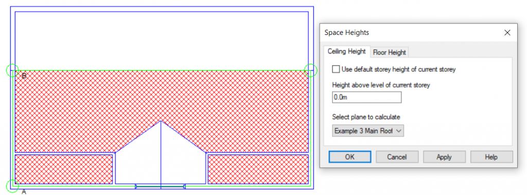
The answer depends on whether or not the roof is on a separate storey. In the case where the internal walls extend upwards to meet the underside of the sloping roof, the best option is to use 3D Planes. But if there is a separate roof space and the internal walls only extend to the underside of a flat ceiling, we should model the roof on a separate storey and the “Set Point Height Option” can be used.

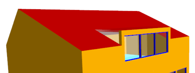
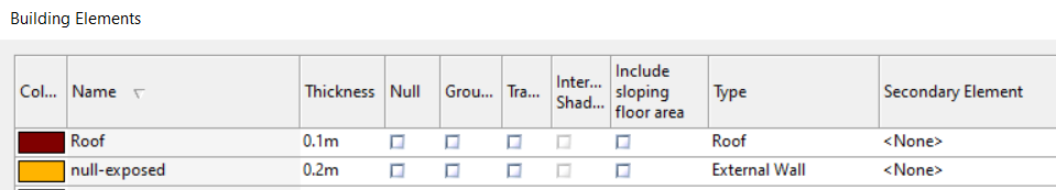
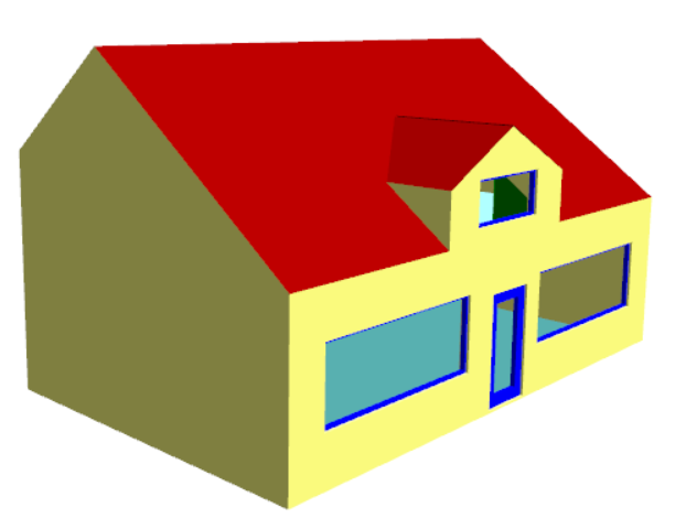
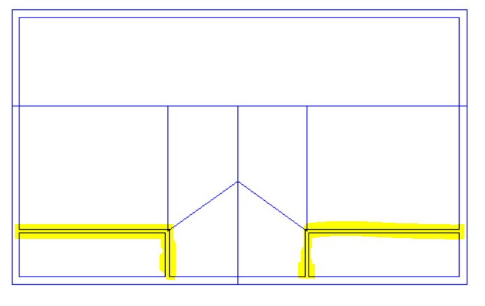
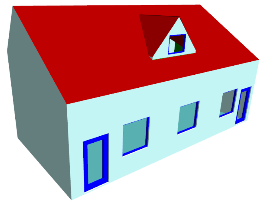
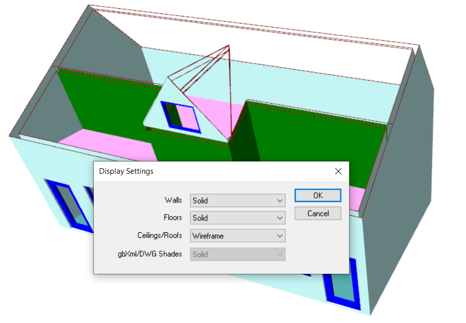
What about “gaps” in the roof where internal walls or null lines are exposed?

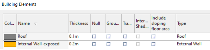
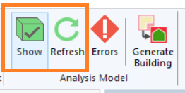
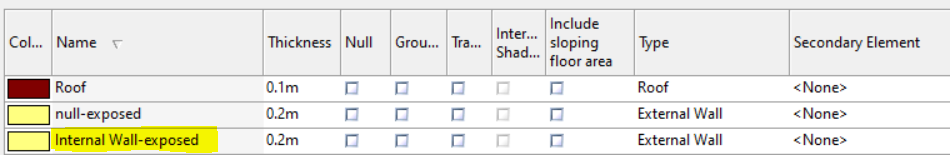
When you create the analysis model, Tas3D creates a new building element for the exposed parts of internal walls, null walls, etc. These new elements, which will have a name ending in “-exposed” can be changed by the user to represent external walls (or, depending on your building, you may want to set these up to represent, e.g., glazing). When you refresh the analysis model you will see that your roof “gaps” have been filled. Be sure to assign an appropriate construction to these building elements in the TBD.

Overview of a 90.1 Appendix G Project in Tas

This blog post gives a brief overview of the methods recommended in Tas to carry out an ASHRAE 90.1 Appendix G analysis. Please note that the emphasis here is on the Tas methods, rather than interpretation of the regulations; as Tas files allow editing, a wide range of different interpretations can be allowed for. Moreover, the exact requirements for results or methods can vary from project to project. The steps explained here are designed to make carrying out a 90.1 project as quick and accurate as possible.

First step: Create the Proposed Tas3D file

When zoning the model, consider space use and conditioning so that each area can receive the correct internal condition and HVAC. Also consider perimeter zoning rules for the version of 90.1 you are using.

Create the Proposed TBD file

The Proposed TBD file represents the building fabric and space use of the designed building (with some important exceptions), and is used as the basis for the Baseline buildings.
Depending on the requirements of your project, may have to consider the following:
Blinds or shades that are controlled automatically or which are permanent features may be included in the Proposed building. Manually controlled blinds or shades cannot be included in the Proposed building.
The building is required to be mechanically ventilated for the purposes of the 90.1 project, so apertures for naturally ventilated areas should be removed even if they are part of the design.
The solar reflectance of roof constructions should be set as 0.30.
Automatic lighting controls may be included, but manual lighting controls may not.
If the lighting system has been designed then you should use these values. If not then the Proposed building should be set based on the building area method for the appropriate building type (more on this later).
EDSL recommend that the fresh air ventilation rate is set correctly in the internal conditions (or at least close to the correct rate) in order to ensure accurate results in TPD.

Add Proposed files to the NPO Studio

The 90.1 Studio allows organisation of the files associated with the project, and has built-in tools to speed up the project work.

Create the Baseline buildings

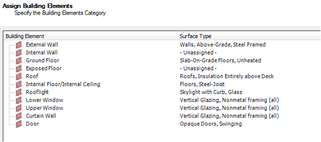
The 90.1 Studio creates the geometry for the four Baseline buildings; this includes rotating the building and applying new constructions in line with 90.1 versions 2007, 2010, 2013, and 2016. Constructions will be applied to the Baseline according to the surface type which the user assigns to the building elements from the proposed TBD file, according to the space use types (also assigned by the user), and according to the climate zone.

Adjust Baseline lighting

The 90.1 Studio adjusts the lighting level in the Baseline TBD files to comply with 90.1 2007, 2010, 2013, or 2016. If the Proposed building uses the building area method (because the lighting system has not been fully designed) then so should the Baseline building. In other cases, use the space-by-space method to assign the lighting gains to the Baseline building.
Lighting controls are not allowed in the Baseline building, and are automatically removed by the lighting wizard.

Simulate the TBD files

The TSD files created by these simulations will be automatically stored within the 90.1 project structure.

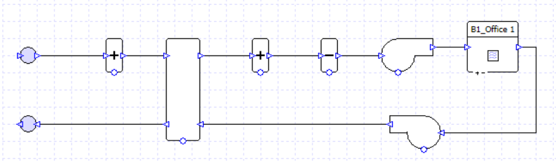
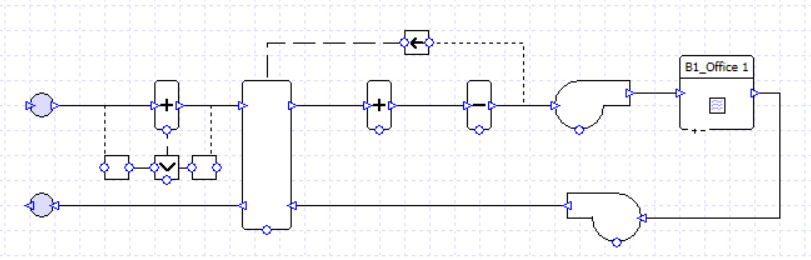
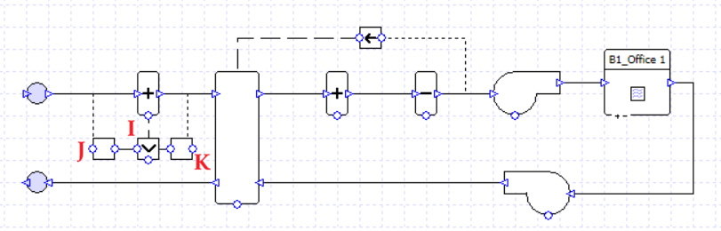
Create the Proposed systems file

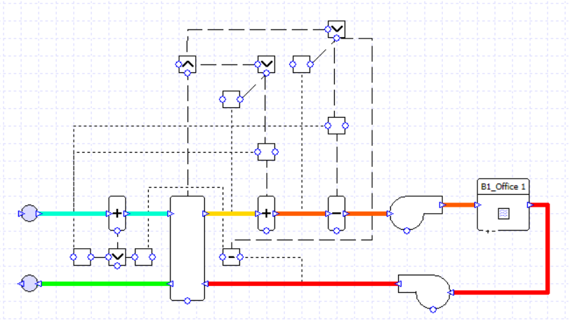
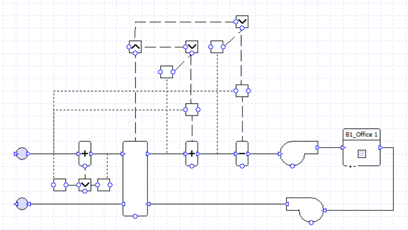
In the Proposed building, if an area of the building has a fully designed mechanical ventilation system which provides both heating and cooling, then you should model the designed system. In all other cases (for example if the area is intended only to be heated, or it is intended to have heating and cooling but the system has not been designed) you must use the appropriate Baseline system.
When modelling the designed system, you should try to replicate the design as closely as possible. In most cases a close equivalent can be found in the wizard and edited later if necessary. Baseline systems can be created in the wizard.
See the Tas documentation for more information on Tas Systems:
https://docs.edsl.net/tpd/
If Baseline systems are used, the user should follow the guidelines below, and ensure that they run the 90.1 airside and plant efficiency tools in the Proposed TPD:
https://docs.edsl.net/NPOTPDx/
When the Proposed TPD is complete, save and add it to the 90.1 Studio.

Complete a sizing run for the Proposed TPD

This is needed so that the zone fresh air rates can be sized (if applicable) and copied to the Baseline TPD files. Save the Proposed TPD after the sizing run.

Create the Baseline 000 TPD file

We only need to create systems for one Baseline building. The TPD files for the three remaining orientations will be generated from this file.
See the guide “Tas Systems Project Wizard and 90.1 Baseline Systems” for details of Baseline system selection and setup:
https://docs.edsl.net/NPOTPDx/
Tas can generate Baseline systems for 90.1 versions 2007, 2010, 2013, 2016, or 2019.
When the Baseline TPD is complete, save and add it to the 90.1 Studio.

Create the other Baseline TPD files

Select the Baseline 000 TPD file. Select the “Use for Baseline Systems” option.

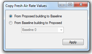
Copy fresh air rate values

Located in the 90.1 Studio under Tools -> Copy Fresh Air Rate Values.
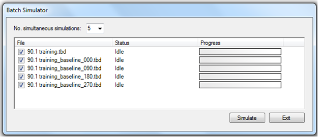
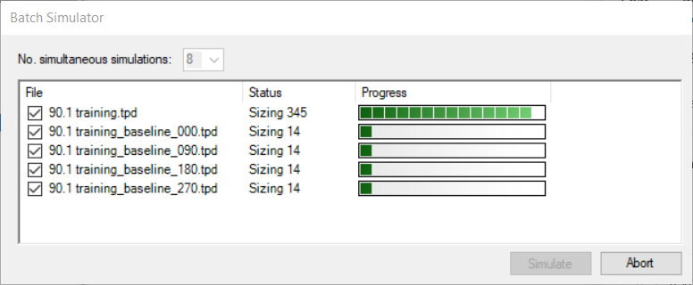
Simulate TPD files

Final Step: Re-runs and reports

The “Generate Documentation” button in the 90.1 Studio creates several reports, including a summary of unmet hours in the Proposed and Baseline buildings. Depending on the 90.1 version and the requirements of your project, a large number of unmet hours may require you to make changes to your system sizing.

A large number of unmet hours could mean zones have been grouped together incorrectly, e.g. zones with very different schedules or gains. It could also indicate airside schedule issues, for example a radiator which is turned off during unoccupied hours and cannot provide out-of-hours heating.

Many 90.1 project submissions are assisted by providing supporting documentation to explain the project inputs. A great deal of this information can be extracted from the systems files, using the “Create Report” button in TPD and by copying data from the 90.1 efficiency tools.