Creating Tas models with Rhino & Honeybee
Rhinoceros, otherwise known as Rhino3D, is a freeform surface modeller that is gaining popularity amongst energy modellers and architects for its ease of use in creating complex geometries. Not only that, but Rhino has a diverse range of plugins which make it possible to perform building energy analysis using interoperability with simulation engines such as Tas. In this blog post, we’ll walk through using the Honeybee plugin by Ladybug tools to link Rhino and Tas.
What are Grasshopper, Ladybug Tools & Honeybee?
Ladybug tools is a collection of applications that support environmental design founded in 2012. These applications are opensource, and are free to use.
One of these tools is called Honeybee, and this tool is a plugin for Grasshopper, a parametric modelling tool which is part of Rhino.
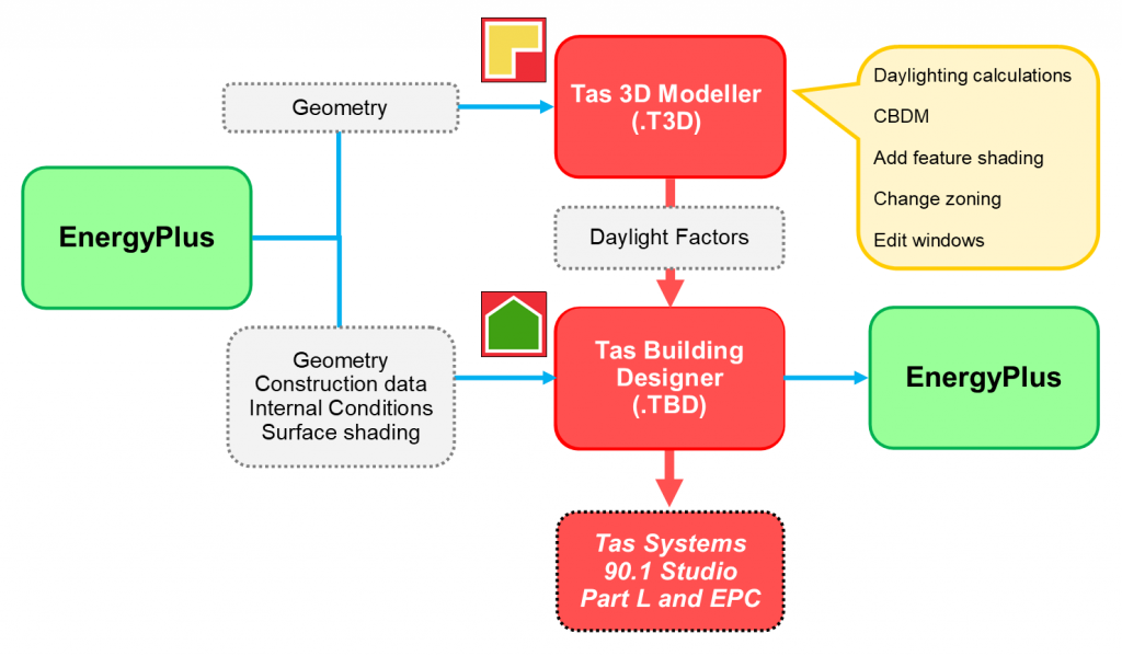
Honeybee can be used to perform daylight simulations using Radiance, and simulate energy models using OpenStudio and EnergyPlus. Honeybee can also be used to produce IDF and gbXML files, both of which provide a route into Tas.
gbXML? IDF? What's the difference?
Both gbXML and IDF are industry standard formats that are designed to allow building design software to share and communicate data. Whilst most building design packages can export gbXML, very few produce gbXML files that contain more than just geometry.
Fortunately, IDF files often contain both geometry and the data required to perform a full building simulation. IDF files produced using Honeybee contain geometry, internal conditions, construction information, design conditions and more, so we recommend using IDF files unless you’re only interested in importing Rhino geometry into Tas.
How do I get started?
In order to get started with Rhino and Honeybee, you’ll first need to download and install Rhino. At the time of writing, you can get an 90 day trial if you do not have a license.
Next, you’ll need to download and install Ladybug tools from Food4Rhino. This is a zip file, so unzip it and start Rhino. Then launch Grasshopper, and open the installer.gh file within Grasshopper:
After running the installation script and restarting Rhino, you should see the Ladybug tools appear in Grasshopper.
Note that you will also need to install OpenStudio if you want to generate IDF files.
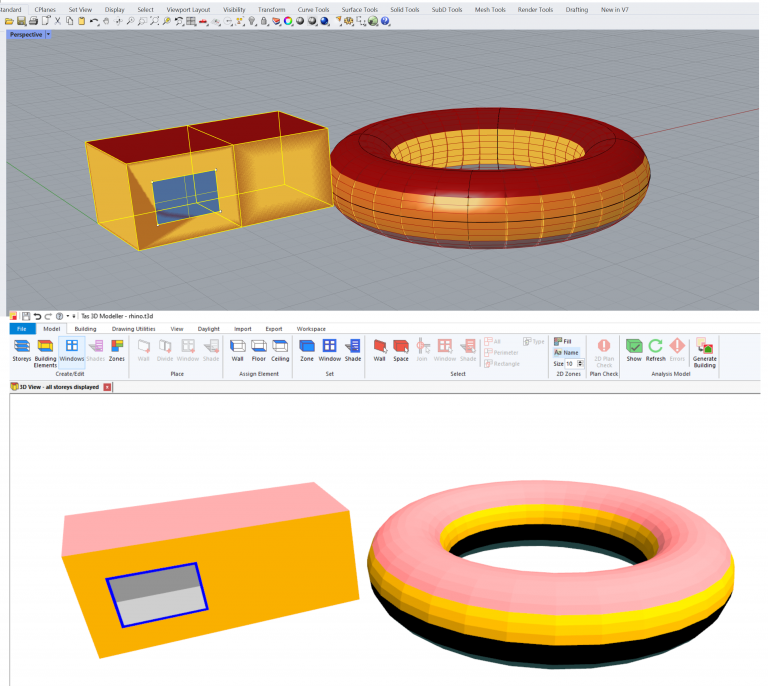
Creating Rhino Geometry
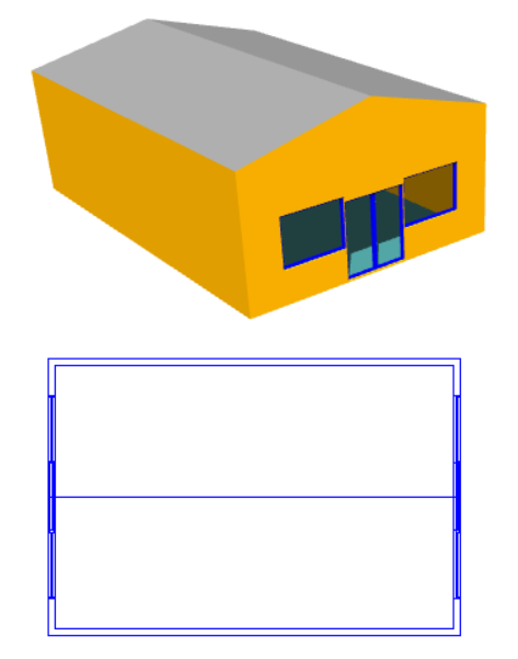
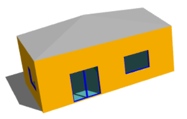
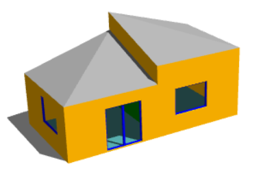
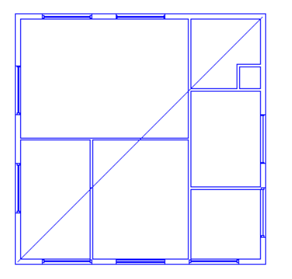
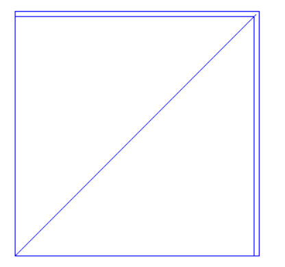
Now we’re ready to create some simple geometry in Rhino, to get ready for export. Let’s start by drawing a two zone model with a couple of windows – this way we can check that our adiabatic links are created correctly, and we’ll be able to see the principles behind marking surfaces as windows. Note that there are several ways to achieve the same outcome in Rhino, so feel free to experiment!
In the video below, I demonstrate how to:
- Set the Rhino units
- Draw two connected cuboids
- Draw surfaces where the windows will be
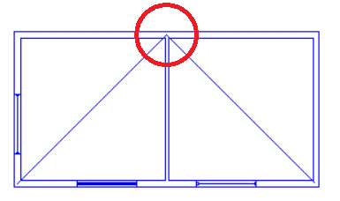
It is important to remember that two touching faces must have the same dimensions in order to form an adiabatic link when using Honeybee.
Setting up Honeybee in Grasshopper
Now that we’ve installed Honeybee and created some geometry in Rhino, we can start setting up our Grasshopper document. In the below video, I demonstrate how to produce a gbXML and an IDF file. I also demonstrate how to modify one of the Honeybee components to produce the IDF file without simulating the OpenStudio project..which saves a lot of time!
To skip running the open studio project and copy the IDF file to a directory of our choice, we can find the line containing run_idf and comment it out using a # at the start of the line.
					import shutil
        elif run_ in (1, 3):  # run the resulting idf throught EnergyPlus
            shutil.copyfile(idf,_idfPathOut)
            #sql, zsz, rdd, html, err = run_idf(idf, _epw_file, silent=silent)

    # parse the error log and report any warnings
#    if run_ in (1, 3) and err is not None:
#        err_obj = Err(err)
#        print(err_obj.file_contents)
#        for warn in err_obj.severe_errors:
#            give_warning(ghenv.Component, warn)
#        for error in err_obj.fatal_errors:
#            raise Exception(error)
We have also used shutil.copyfile to copy the IDF file to the path of our choosing using the _idfPathOut parameter we added to the ModelToOSM component. For full details, see the video above.
Commenting out the end of the script stops any error messages appearing when we attempt to run the component.
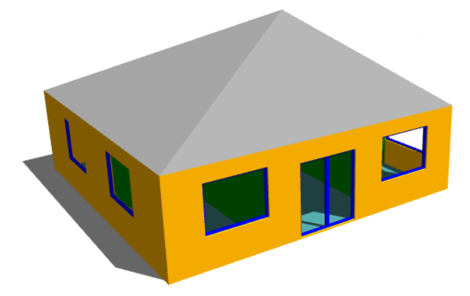
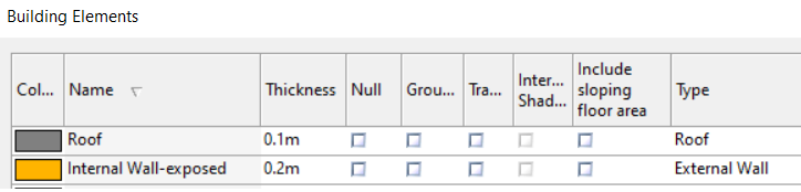
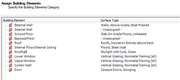
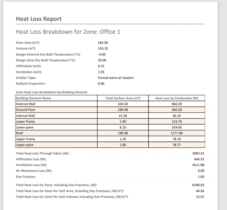
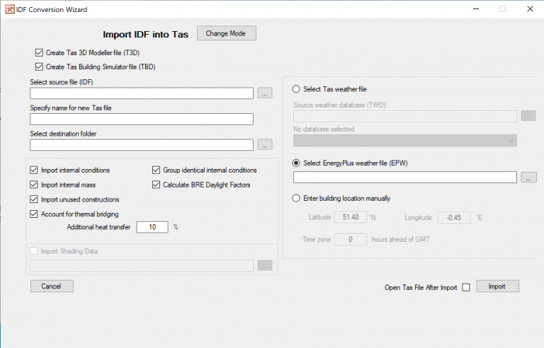
Importing the IDF into Tas
Once we’ve created our IDF file, we can import it into Tas using the IDF tool. We can optionally create a Tas3D model for shading calculations, import constructions & geometry and even specify the weather we want to use to simulate. In other words, the model is ready to go!
Rhino to Tas Workflow Summary
Below is a labelled Grasshopper diagram showing the key steps in creating gbXML and IDF files from Rhino. Remember, this is just one way to do it! Some of the components can be linked together in a different order, and some can be omitted. If you wanted to model % glazing, for example, you could add the apertures straight to the HoneyBee model and skip specifying and combining them.
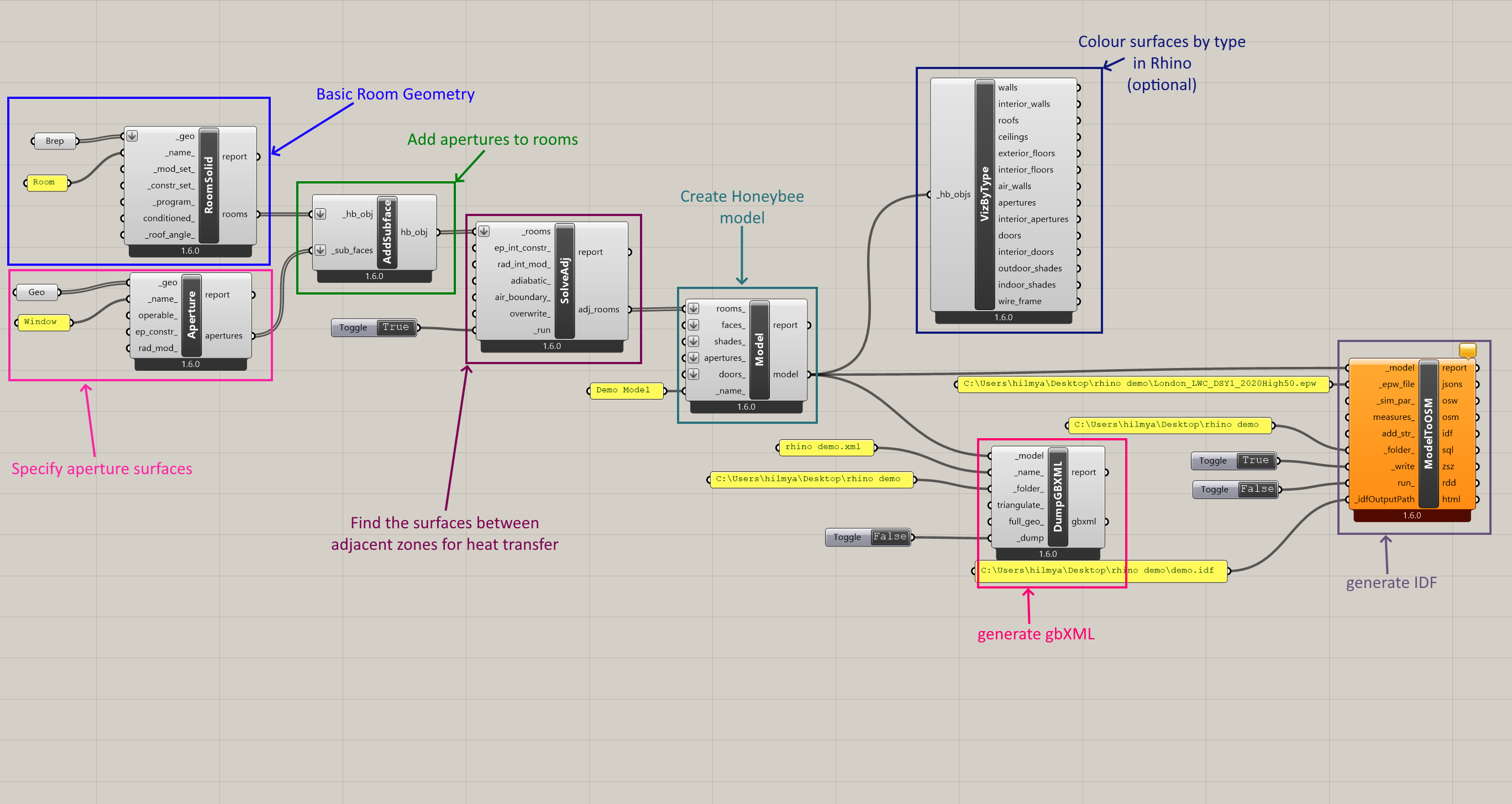
As the Rhino files are saved separately to the Grasshopper files, you can save the Grasshopper files and re-use them on future projects just by updating the geometry components each time.
What else is Possible with Tas & Rhino?
As Grasshopper provides a visual programming interface to Rhino and Tas has a programming interface, the two can be linked to achieve endless outcomes – from parametric runs to performing full energy simulations and visualising the results in Rhino.
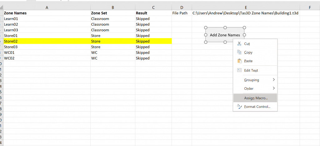
You can create your own Tas Grasshopper code modules via python scripts:
					import win32com.client

#open the building simulator and then open a file
tbdDoc = win32com.client.Dispatch("TBD.Document")
tbdDoc.openReadOnly("C:\\Users\\hilmya\\Desktop\\tas house.tbd")

i = 0
while(tbdDoc.Building.getZone(i) is not None):
    #print each zone name to console
    print(tbdDoc.Building.getZone(i).name)
    i = i+1
Better yet, you can create C# modules in Grasshopper which have the advantage of code completion:
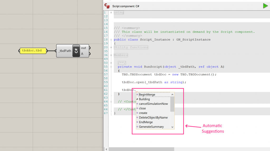
In order to use the Tas automation interface with a c# script component in Grasshopper, right click on the component and click Manage Assemblies. Then reference the appropriate dll, for example, for TBD you would reference Interop.TBD.dll from the Tas installation directory.
You can do the same with the Visual basic (VB script) component.