Learn to Code with Tas and Excel Lesson 3- Tas3D Zone Writer pt 2
In the last lesson, we created a macro that added zone names from an Excel spreadsheet to a 3D modeller file. Specifically, it:
- Opened the 3D modeller
- Opened an existing Tas3D file
- Added a new zone group
- Read the names of zones from the spreadsheet and added them as new zones to the new zone group
- Saved and closed the file
In this lesson, we’ll continue where we left off and add some extra functionality to our macro. We’d like to extend our macro to:
- Check for duplicate zone names
- Sort the new zones into zone groups
- Read the existing zones in the file
So lets dive in.
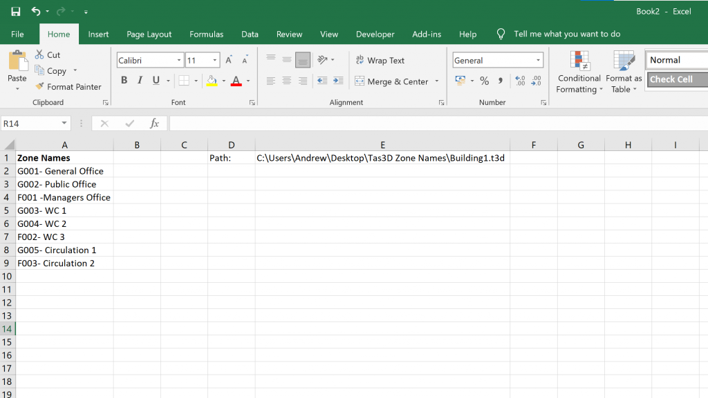
Before we can start modifying our macro from the previous lesson to deal with duplicate zones and zone sets, we need to add a couple of columns to our spreadsheet so we’re on the same page:
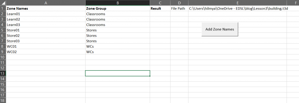
We need to add a heading to column B so we can use it for zone sets, another heading for column C so the macro can report whether it added the zone, and some sample zone names and zone set names.
Checking for duplicate zone names
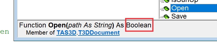
To check for duplicate zone names, we’ll write a function that returns a Boolean (True/False) depending on whether a Tas3D file already contains a zone with that name.
Lets take a look at the script for our function:
					Function ZoneExists(name As String, doc As TAS3D.T3DDocument) As Boolean

    'declare variables for our loop
    Dim curZoneIndex As Integer
    Dim curZone As TAS3D.Zone

    'set the initial zone index to 1
    curZoneIndex = 1

    'go through each zone in the building
    While Not doc.Building.GetZone(curZoneIndex) Is Nothing

        'set the curZone reference variable to the current zone
        Set curZone = doc.Building.GetZone(curZoneIndex)

        'if the zone has the name we are looking for, return true
        If curZone.name = name Then
            ZoneExists = True
            Exit Function
        End If

        'increment the zone index so we look at the next one in the file
        curZoneIndex = curZoneIndex + 1
    Wend

    'if we have checked all the zones and none match the name we are looking for, return false
    ZoneExists = False

End Function
This function a while loop to iterate over every zone in a Tas3D file, checking to see if the name of each zone matches the name passed into the function as a parameter.
If the function finds a zone with the name it is looking for, it immediately returns True.
If the function searches through all the zones and does not find the name it is looking for, it returns False.
For more information about Functions, see the section at the end of lesson 1.
Function breakdown: how does it work?
We’ll start by looking at the definition of our function:
					Function ZoneExists(name As String, doc As TAS3D.T3DDocument) As Boolean

    'Code goes here

End Function
Here, we have created a function called ZoneExists. This function has two parameters – the name of the zone we are looking for which is of type String, and the doc which is a reference variable to a Tas3D Document. The ‘As Boolean’ after the parameters is the return type of the function. This means when we call (use) the function, the function can return True or False.
					    'declare variables for our loop
    Dim curZoneIndex As Integer
    Dim curZone As TAS3D.Zone

    'set the initial zone index to 1
    curZoneIndex = 1
Next, we declare some primitive and reference variables we will use when we are looking through each of the zones in the Tas3D document, inside our while loop. We have an integer called curZoneIndex to track the number of the zone we are currently examining, and we have a reference variable of type Tas3D.Zone called curZone, so we can more easily refer to the zone we are currently checking the name of.
We also have to initialise the curZoneIndex variable to 1 (line 6), because in Tas3D, the first zone is assigned the number 1.
					'go through each zone in the building
    While Not doc.Building.GetZone(curZoneIndex) Is Nothing

        'set the curZone reference variable to the current zone
            'TODO

        'if the zone has the name we are looking for, return true
            'TODO

        'increment the zone index so we look at the next one in the file
        curZoneIndex = curZoneIndex + 1
    Wend
Next comes the basic structure of our while loop; on line 1, we check to see whether the zone in the building with index = curZoneIndex exists. Remember, the condition of the while loop and the code within it run multiple times when the condition is true. Before we enter the loop for the first time, we are checking to see whether the first zone in the building exists. If it does not, the body of the while loop (lines 3-11) doesn’t get executed.
Assuming we do enter the while loop, on line 11 we increment our curZoneIndex by 1 so that when the loop repeats, we check the next zone in the file. We’re now ready to fill in the rest of the functionality of the while loop, which have TODO comments on lines 5 and 8.
					'go through each zone in the building
    While Not doc.Building.GetZone(curZoneIndex) Is Nothing

        'set the curZone reference variable to the current zone
        Set curZone = doc.Building.GetZone(curZoneIndex)

        'if the zone has the name we are looking for, return true
        If curZone.name = name Then
            ZoneExists = True
            Exit Function
        End If

        'increment the zone index so we look at the next one in the file
        curZoneIndex = curZoneIndex + 1
    Wend
On line 5, we set our curZone reference variable to the zone in the document with the index equal to curZoneIndex.
On line 8, we check to see if the name of that zone matches the name we passed into our function. If it does, we set the return value of the function to true (line 9), and exit the function early as we no longer need to examine any more zones.
					    'if we have checked all the zones and none match the name we are looking for, return false
    ZoneExists = False
Finally, if we complete our while loop without finding a zone with a name that matches the one we’re looking for, we set the return value of the function to False to indicate a zone with that name does not exist in the file.
Finding existing Zone Sets
Lets quickly review the flow of our macro as it stands. Currently, it adds every new zone to a single zone set, which it creates before looking through the list of new zone names on the worksheet.
If we were to modify our macro so it added a new zone set for each new zone, we have a potential problem. If we had multiple zones that were supposed to belong to the same zone set we’d end up making multiple zone sets with the same name!
To overcome this problem, we need to create a function that looks through the zone sets currently in the file to see if there’s already one with the name we need. If there is, we need a reference to it so we can add zones to it. If there isn’t, we know we need to add a new zone set to the file.
Lets see what such a function could look like:
					Function GetZoneSet(name As String, doc As TAS3D.T3DDocument) As TAS3D.zoneSet
    Dim curZoneSetIndex As Integer
    Dim curZoneSet As TAS3D.zoneSet
    curZoneSetIndex = 1

    While Not doc.Building.GetZoneSet(curZoneSetIndex) Is Nothing

        'set the current zone set reference to the next zone set
        Set curZoneSet = doc.Building.GetZoneSet(curZoneSetIndex)

        'check to see if the name matches what we're looking for. If it does, return the zone set.
        If curZoneSet.name = name Then
            Set GetZoneSet = curZoneSet
            Exit Function
        End If

        'increment the index so we look at the next zone set when the loop repeats
        curZoneSetIndex = curZoneSetIndex + 1
    Wend

    'If we finish the loop without finding the zone set, return nothing
    Set GetZoneSet = Nothing

End Function
This function works in a similar way to the ZoneExists function. The return type is different, and rather than iterating through every zone in the building we iterate over every zone set.
Function breakdown: How does it work?
We start by declaring our functions name, parameters and return type:
					Function GetZoneSet(name As String, doc As TAS3D.T3DDocument) As TAS3D.zoneSet

    'function code goes here

End Function
This function is called GetZoneSet, its parameters are a name as a string and doc which is a reference to the Tas3D.T3DDocument we wish to search through. The function returns a reference variable to a Tas3D.zoneSet; if it doesnt find one, it returns nothing.
					Dim curZoneSetIndex As Integer
Dim curZoneSet As TAS3D.zoneSet
curZoneSetIndex = 1
We start by defining some variables we’ll use while we’re looking through all the zoneSets in the file. We use the curZoneSetIndex integer variable to keep track of the index of the zoneSet we are currently working with. The first zoneSet in a Tas3D document is given an index of 1, so we must set the initial value of our curZoneSetIndex to 1.
We use the curZoneSet reference variable to refer to the current zoneSet.
					While Not doc.Building.GetZoneSet(curZoneSetIndex) Is Nothing

    'set the current zone set reference to the next zone set
    'TODO

    'check to see if the name matches what we're looking for. If it does, return the zone set.
    'TODO

    'increment the index so we look at the next zone set when the loop repeats
    curZoneSetIndex = curZoneSetIndex + 1
Wend
On line 1, we check to see if there is a zone set in the Tas3D document we passed in as a parameter with an index equal to curZoneSetIndex. If there is a zone set, GetZoneSet will return something (rather than nothing), and we will enter the while loop.
Before we reach the Wend of the while loop and the condition on line 1 is re-evaluated, we increment the curZoneSetIndex by 1 so we look at the next zone set in the file. If there is no zone set with that index, GetZoneSet returns nothing so we do not enter the while loop again.
					While Not doc.Building.GetZoneSet(curZoneSetIndex) Is Nothing

    'set the current zone set reference to the next zone set
    Set curZoneSet = doc.Building.GetZoneSet(curZoneSetIndex)

    'check to see if the name matches what we're looking for. If it does, return the zone set.
    If curZoneSet.name = name Then
        Set GetZoneSet = curZoneSet
        Exit Function
    End If

    'increment the index so we look at the next zone set when the loop repeats
    curZoneSetIndex = curZoneSetIndex + 1
Wend
On line 4, we set our zoneSet reference variable to the zone set with index curZoneSetIndex.
On line 7, we check to see if the name of that zone set matches the one we’re looking for that we passed in as a parameter. If it does, on line 8 we set the return value of the function to the currentZoneSet and on line 9 we exit the function early so we don’t consider any more zone sets.
					'If we finish the loop without finding the zone set, return nothing
Set GetZoneSet = Nothing
Finally, if we have passed the end of the while loop without finding the zone set with the name we are looking for, we set the return value of the function to nothing.
Putting it all together
Now that we’ve written our new functions to check for existing zone names and zone sets, we are ready to modify our existing macro to sort the new zones into zone sets. I’ve highlighted some of the main changes.
					Sub AddZoneNames()
    'Read the file path from the spreadsheet
    Dim filePath As String
    filePath = Cells(1, 5)

    'Open the 3D modeller
    Dim t3dApp As TAS3D.T3DDocument
    Set t3dApp = New TAS3D.T3DDocument

    'Declare a variable for checking if operations were successful
    Dim ok As Boolean

    'Try to open the existing file
    ok = t3dApp.Open(filePath)

    'Check if it did open successfully
    If Not ok Then
        MsgBox "Couldnt open the file; is it in use?"
        Exit Sub
    End If


    'Define our loop variables
    Dim rowIndex As Integer
    Dim zoneName As String
    Dim zoneSetName As String
    Dim zoneSet As TAS3D.zoneSet
    Dim newZone As TAS3D.Zone

    'Set the starting rowIndex
    rowIndex = 2

    'Check each zone name cell to see if it contains something
    While Not IsEmpty(Cells(rowIndex, 1))

        'Read the zone name from excel
        zoneName = Cells(rowIndex, 1)

        'Read the zone set name from excel
        zoneSetName = Cells(rowIndex, 2)

        'Check that zone name isnt already in use
        If ZoneExists(zoneName, t3dApp) Then
            Cells(rowIndex, 3) = "Skipped"
        Else

            'Get the zone set if it exists
            Set zoneSet = GetZoneSet(zoneSetName, t3dApp)

            'If it doesnt exist, make a zone set with that name
            If zoneSet Is Nothing Then
                Set zoneSet = t3dApp.Building.AddZoneSet(zoneSetName, "", 0)
            End If


            'Add a zone to the zone set
            Set newZone = zoneSet.AddZone()

            'Change the name of the zone we just added
            newZone.name = zoneName

            'Note that the addition was a success
            Cells(rowIndex, 3) = "Added"

        End If

        'Increment the row index (so we read the next cell down)
        rowIndex = rowIndex + 1
    Wend

    'Save the file and check the save was successful
    ok = t3dApp.Save(filePath)

    If Not ok Then
        MsgBox "Couldn't save the file!"
        Exit Sub
    End If

    'Close the file
    t3dApp.Close

    'Close the 3D modeller
    Set t3dAppp = Nothing

    'Message box, so we know when it's done running
    MsgBox "Finished!"

End Sub
Rather than use a fixed name for the new zone set, we read the zone set name from the worksheet:
					    'Read the zone set name from excel
    zoneSetName = Cells(rowIndex, 2)
Before we check to see whether a zone set exists with this name, we should check to see if a zone already exists with this name. Why? Because if we check after we’ve already created a new zone set, we might end up making an empty zone set and then realising we have no zone to put in it as a zone with that name already exists in a different zone set!
					'Check that zone name isnt already in use
If ZoneExists(zoneName, t3dApp) Then
    Cells(rowIndex, 3) = "Skipped"
Else

  ' ... code to add the new zone & zone set ...

End If
On line 2, we are calling our ZoneExists function as the condition to an if statement with the zoneName we read from the spreadsheet and a reference to our Tas3D document. If the function returns true, this means a zone with that name already exists in the 3D file. We therefore write the message “Skipped” next to that row in the spreadsheet so the user is notified that there was a problem.
If ZoneExists returns false, this means there is no zone with that name in the file already so we can create it and add it.
					        'Check that zone name isnt already in use
        If ZoneExists(zoneName, t3dApp) Then
            Cells(rowIndex, 3) = "Skipped"
        Else

            'Get the zone set if it exists
            Set zoneSet = GetZoneSet(zoneSetName, t3dApp)

            'If it doesnt exist, make a zone set with that name
            If zoneSet Is Nothing Then
                Set zoneSet = t3dApp.Building.AddZoneSet(zoneSetName, "", 0)
            End If


            'Add a zone to the zone set
            Set newZone = zoneSet.AddZone()

            'Change the name of the zone we just added
            newZone.name = zoneName

            'Note that the addition was a success
            Cells(rowIndex, 3) = "Added"

        End If
On line 7, we use our GetZoneSet function to search through the Tas3D document and look for a zone set with the name we desire. If it finds one, our zoneSet reference variable is set to a valid reference to that zone set.
If GetZoneSet cannot find one, the zoneSet variable will reference Nothing, so we check for this on line 10. If it is equal to nothing, we know we need to add a new zone set and name it, so this is what we do on line 11.
By the time we get to line 16, the zoneSet variable should refer to a valid zone set. We can therefore add a new zone to that zone set, and set the name.
On line 22, we leave a comment that the addition was successful, so the user knows that zone was added to the file.
Details: "Nothing"
In previous lessons, we discussed Primitive and Reference variables. Primitive variables must always have a value; if we define a new primitive variable and do not set its value, it will have a default value:
Dim number as integer 'The default value is 0
Reference variables may not always point to a valid object, and may point to Nothing. This is the default value for reference variables:
					Dim someText as String 'Default value is Nothing
Dim doc as Tas3D.T3DDocument 'Default value is Nothing
We should therefore be aware that functions that return reference variables may sometimes have values of Nothing. We must check for this, because if we try to call a function that belongs to the type the reference variable controls and the reference variable controls Nothing, we’ll get an error and our program will break.
When we test for nothing, we cannot use the equals operator – we have to use the is keyword
					Dim doc as Tas3D.T3DDocument() 'default value is Nothing

'Check for nothing
If doc Is Nothing Then
    'doc is an invalid reference
End If

'Check for something
If Not doc Is Nothing Then
    'doc is a valid reference
End If
For more information about the Nothing value, see this page.
Next Lesson
We haven’t really introduced anything new in this lesson, we’ve just been using the concepts introduced in previous lessons. This is great news, as it means we have already covered a lot of the programming basics.
In the next lesson, we’ll discuss how we can modify our macro to make it faster for large files.