Rhino to Tas: Grasshopper

Rhino to Tas: Grasshopper Scripts

In the last Rhino To Tas blog post, we looked at how we can use LadybugTools Honeybee grasshopper plugin to generate gbXML and IDF files that can be imported into Tas. We also touched on how we could automate Tas from within Grasshopper by writing scripts. 

In this post, we’ll expand on this work and go through some examples of how we can manipulate Tas files from Grasshopper, and how we can pass data back to Rhino. 
This post is made up of the following sections:

  • Creating a c# script component
  • Referencing the Tas libraries
  • Sample: Import gbXML
  • Sample: Import IDF
  • Sample: Simulate TBD
  • Sample: Read TSD results

Creating a Grasshopper Script Component

Let’s start by learning how to create a c# Grasshopper script. To do so, double click anywhere in the Grasshopper canvas and type in “c# script”:
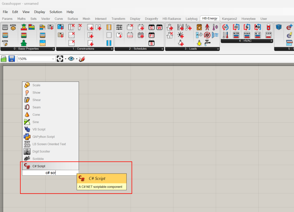
Adding a grasshopper c# script.

Place the c# script component and then zoom in on it. Once you have done so, you will see script inputs on the left and outputs on the right side of the component:
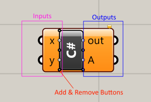
Anatomy of the c# script component in grasshopper, showing inputs and outputs.

If you zoom in enough on the component, you will see plus and minus icons within a circle as per the image above. These are buttons that allow you to add and remove inputs and outputs from the component. 

You can also rename inputs and outputs by right clicking on the name of the input or output and editing the text directly in the menu that appears:
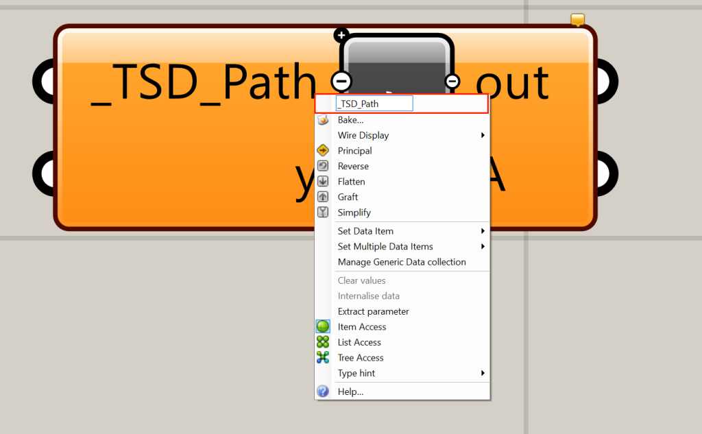
Right click menu that appears when right clicking in an input label on the c# component in grasshopper.

Now that we have placed a script component and have named some input/output variables, we can double click on the component to edit the script:
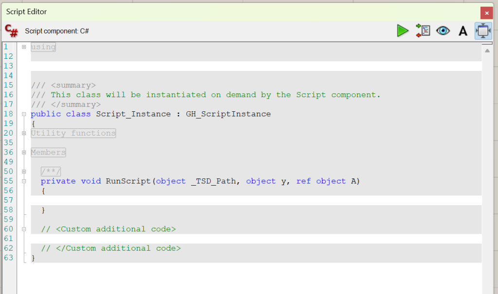
As you can see, the _TSD_Path variable we named on the component appears as an input to the RunScript function, and the outputs are also variables passed by reference. Passing by reference means that something may use the value of the variable outside of that function – which is exactly what we would expect with an output variable. 

You will also notice that most of the lines in the script editor are grey – these are lines we cannot edit or change. We can define new functions outside RunScript in the ‘Custom Additional Code’ section and we can call those functions from within the RunScript function.

Adding Library References

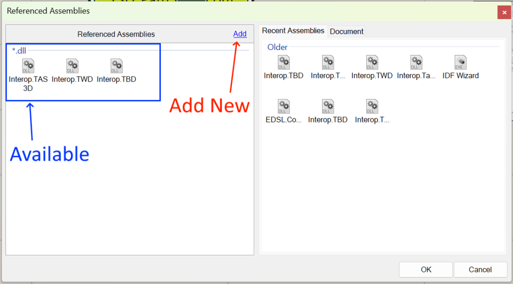
If we want to be able to control Tas from our Grasshopper script so that Grasshopper knows what , for example, a TSD Document is, we need to reference the Tas interoperability libraries. To do so, right click on the c# script component and select Manage Assemblies:
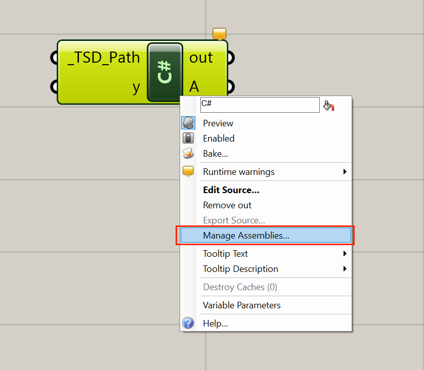
c# component context menu showing manage assemblies button.

The Tas libraries can be found in the Tas installation directory, and have names like:

  • Interop.TAS3D.dll    <- 3D Modeller
  • Interop.TSD.dll         <- Results Viewer
  • Interop.TBD.dll        <- Building Simulator

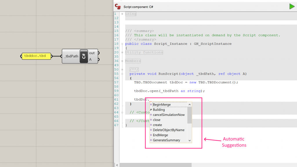
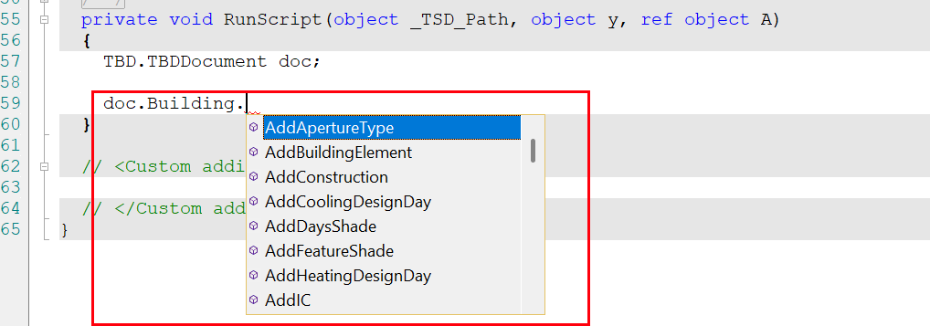
Once these have been reference, you’ll see intellisense style auto-complete suggestions when writing scripts:
Sample: Importing gbXML

This sample script demonstrates how to automatically import a gbXML file into Tas3D. You’ll need to reference the Interop.Tas3D.dll as described in the previous section for this component to function.
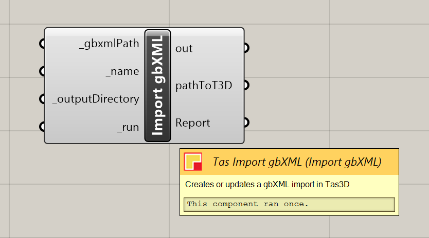
custom grasshopper c# script component showing import gbXML into Tas 3D modeller.
				
					  private void RunScript(object _gbxmlPath, object _name, object _outputDirectory, object _run, ref object pathToT3D, ref object Report)
  {
    //null check on the required inputs
    if (_gbxmlPath == null || _name == null || _outputDirectory == null || _run == null)
    {
      Report = "One or more required inputs are not specified";
      return;
    }

    //cast the inputs to their expected types
    string gbxmlPath = (string) _gbxmlPath;
    string name = (string) _name;
    string outputDirectory = (string) _outputDirectory;
    bool run = (bool) _run;
    if (!run)
    {
      Report = "Run flag is set to false. Exiting without action.";
      return;
    }

    //check if the gbXML file exists
    if (!System.IO.File.Exists(gbxmlPath))
    {
      Report = "The specified gbXML file does not exist: {gbxmlPath}";
      return;
    }

    //check if the output directory exists, if not create it
    if (!System.IO.Directory.Exists(outputDirectory))
    {
      //add a note about creating the directory
      Report = "The specified output directory does not exist. Creating: {outputDirectory}";
      System.IO.Directory.CreateDirectory(outputDirectory);
    }

    //construct the t3d path
    var t3dPath = System.IO.Path.Combine(outputDirectory, name + ".t3d");

    //open an instance of the 3D modeller
    var doc = new TAS3D.T3DDocument();

    //does the file already exist?
    bool fileExists = System.IO.File.Exists(t3dPath);


    if(fileExists)
    {
      if(!doc.Open(t3dPath)) throw new Exception("Failed to open the t3d. is it in use?");
    }else
    {
      //better create one
      doc.Create();
    }

    //now import the gbXML
    doc.ImportGBXML(gbxmlPath, 1, 1, 1);

    //save and close
    doc.Save(t3dPath);
    doc.Close();

    //report success
    Report = "Successfully imported gbXML file to T3D: {t3dPath}";

    pathToT3D = t3dPath;
  }


Sample: Importing IDF

This sample script demonstrates how to automatically import an IDF file into Tas3D. You’ll need to reference the Interop.Tas3D.dll as described in the previous section for this component to function.

You’ll also need to import the IDF Wizard.exe.
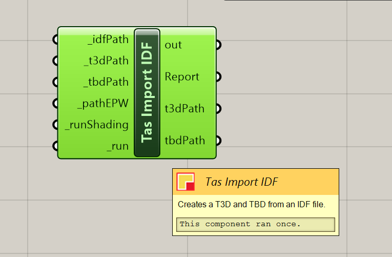
				
					private void RunScript(object _idfPath, object _t3dPath, object _tbdPath, object _pathEPW, object _runShading, object _run, ref object Report, ref object t3dPath, ref object tbdPath)
  {
    //check inputs
    if (_idfPath == null || _t3dPath == null || _tbdPath == null || _runShading == null || _pathEPW == null || _run == null)
    {
      Report = "One or more required inputs are not specified";
      return;
    }

    //cast to their proper types
    string idfPath = (string) _idfPath;
    string t3dPathOut = (string) _t3dPath;
    string tbdPathOut = (string) _tbdPath;
    bool runShading = (bool) _runShading;
    string pathEPW = (string) _pathEPW;
    bool run = (bool) _run;
    if (!run)
    {
      Report = "Run flag is set to false. Exiting without action.";
      return;
    }

    //check if the idf file exists
    if (!System.IO.File.Exists(idfPath))
    {
      Report = "The specified idf file does not exist: {idfPath}";
      return;
    }

    //we have to delete the t3d and tbd if they exist already. merge is not yet supported.
    if(System.IO.File.Exists(t3dPathOut))
    {
      System.IO.File.Delete(t3dPathOut);
    }

    if(System.IO.File.Exists(tbdPathOut))
    {
      System.IO.File.Delete(tbdPathOut);
    }

    var importer = new IDF_Wizard.clsProjectManager(true, true);
    importer.IDFPath = idfPath;
    importer.Options = new IDF_Wizard.clsOptions();
    importer.Options.FilePathEPW = pathEPW;
    importer.Options.WeatherEPW = true;
    importer.Options.InternalConditions = true;
    importer.Options.UnusedConstructions = true;
    importer.Options.Automation = true;


    importer.Import(idfPath, tbdPathOut, t3dPathOut, null);

    if(!runShading )
    {
      //no shading, we are done.
      Report = "Import completed without shading.";
      return;
    }

    //check we have a t3d file now. if not, something probably went wrong.
    if (!System.IO.File.Exists(t3dPathOut))
    {
      Report = "Import failed: T3D file was not created.";
      return;
    }

    //and check for the tbd too
    if(!System.IO.File.Exists(tbdPathOut))
    {
      Report = "Import failed: TBD file was not created.";
      return;
    }

    //ok we better do the shading. open the t3d
    var doc = new TAS3D.T3DDocument();
    if (!doc.Open(t3dPathOut))
    {
      Report = "Failed to open the T3D file for shading. Is it in use?";
      return;
    }

    doc.ExportNew(1, 365, 15, 1, 1, 1, tbdPathOut, 0, 0, 0);

    //report finished
    Report = "Finished.";
    tbdPath = tbdPathOut;
    t3dPath = t3dPathOut;
  }


Sample: Simulating a TBD

This sample script demonstrates how to open and simulate a TBD. You’ll need to reference the Interop.TBD.dll as described in the previous section for this component to function.
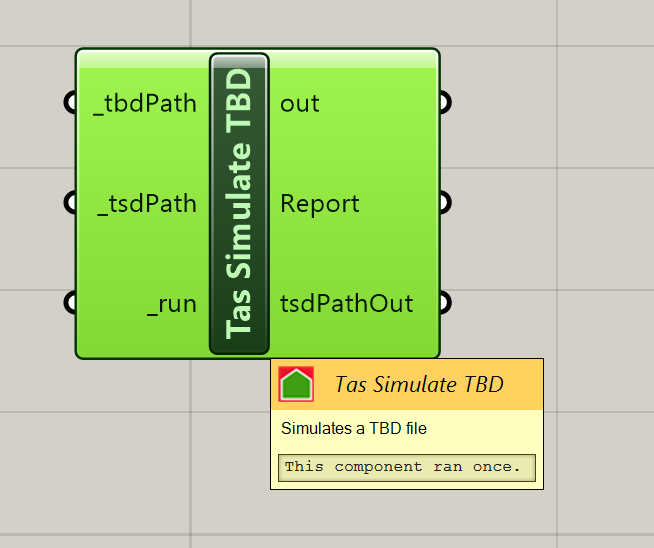
				
					private void RunScript(object _tbdPath, object _tsdPath, object _run, ref object Report, ref object tsdPathOut)
  {
    //check inputs
    if(_run == null || !(bool) _run)
    {
      return;
    }

    //check tbd path
    if(_tbdPath == null)
    {
      Report = "No TBD path specified.";
      return;
    }

    //check tsd path
    if(_tsdPath == null)
    {
      Report = "No TSD path specified.";
      return;
    }

    //cast to proper types
    string tbdPath = (string) _tbdPath;
    string tsdPath = (string) _tsdPath;


    //check if the tbd file exists
    if (!System.IO.File.Exists(tbdPath))
    {
      Report = "The specified tbd file does not exist: {tbdPath}";
      return;
    }

    //open the tbd
    var doc = new TBD.TBDDocument();
    if(doc.openReadOnly(tbdPath) == 0)
    {
      Report = "Failed to open the TBD file. Is it in use?";
      return;
    }

    //export the tsd
    if(doc.simulate(1, 365, 0, 1, 0, 0, tsdPath, 1, 0) == 0)
    {
      Report = "Failed to simuate the TBD.";
      return;
    }

    //report success, return the tsd path
    Report = "Successfully simulated TBD.";
    tsdPathOut = tsdPath;

  }


Sample: Reading a TSD result

This sample script demonstrates how to open a TSD file and read the annual cooling result for all zones. You’ll need to reference the Interop.TSD.dll as described in the previous section for this component to function.
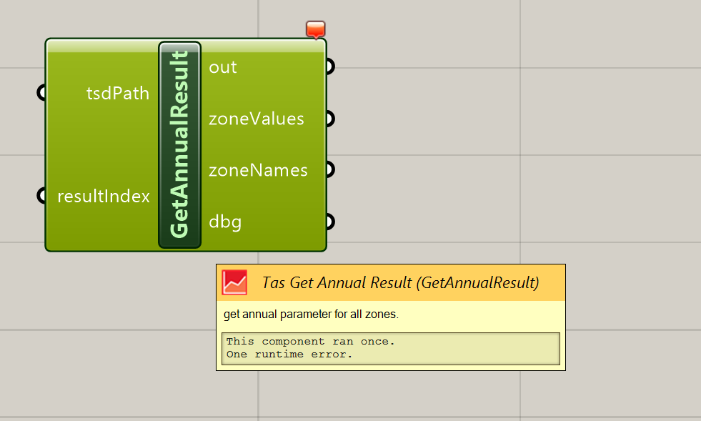
				
					private void RunScript(object tsdPath, object resultIndex, ref object zoneValues, ref object zoneNames, ref object dbg)
  {
    var names = new List<string>();
    var values = new List<double>();


    var resultIndexInt = int.Parse(resultIndex.ToString());

    string strPath = tsdPath as string;
    if (string.IsNullOrWhiteSpace(strPath))
    {
      zoneNames = names;
      zoneValues = values;
      return;
    }

    try
    {
      //open TSD document
      var doc = new TSD.TSDDocument();

      if (!doc.openReadOnly(strPath))
      {
        Rhino.RhinoApp.WriteLine("Failed to open TSD document at path: " + tsdPath);
        zoneNames = names;
        zoneValues = values;
        return;
      }


      //access simulation + building data
      var sim = doc.SimulationData;       
      var bld = sim.GetBuildingData();    

      int zoneCount = bld.zoneCount; 
      Rhino.RhinoApp.WriteLine(zoneCount.ToString());
      for (int i = 1; i <= zoneCount; i++)
      {
        var z = bld.GetZoneData(i);       
        dbg = z.name;
        string name = z.name;         
        float[] val = (float[]) z.GetAnnualSumZoneResult((TSD.tsdZoneArray) resultIndexInt, 1, 365, TSD.tsdResultsPeriod.tsdResultsPeriodAnnual, false);
        dbg = val;
        names.Add(name);
        values.Add(val[0]);

      }
    }
    catch (Exception ex)
    {
      dbg = ex;
      Rhino.RhinoApp.WriteLine("Error accessing Tas TSD: " + ex.Message);
    }

    zoneNames = names;
    zoneValues = values;
    dbg = zoneNames;
  }


Python Scripting in Tas

Python Scripting in Tas

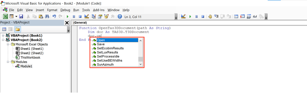
In previous blog posts, we’ve looked at how you can get started with the Tas API. We mentioned that you can use almost any programing language to automate Tas, and I personally recommended getting started with Visual Basic for Applications (VBA) with Microsoft Excel. This is for two reasons; the first, is that an Excel worksheet is a convenient way to store data you might want to put into Tas and get out of Tas. The second, is that using Excel to write Macros requires very little to get started and, most importantly of all, comes with ‘Intellisense’

Intellisense menu for the Tas type library
When you add a period (.) to Tas variables in the visual basic editor, the Intellisense window appears telling you what operations are available for that object

This Intellisense, sometimes known as code completion or auto-complete, is pretty handy as it saves you the trouble of having to refer to online documention and type library information viewers as frequently when you are programming using our API.

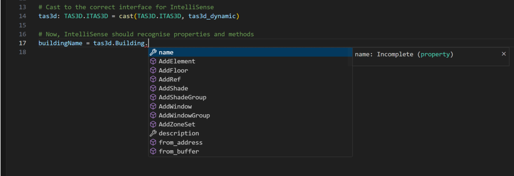
With most Python setups, this Intellisense for Tas is not available, so in this blog post, we’ll walk through how to set it up.

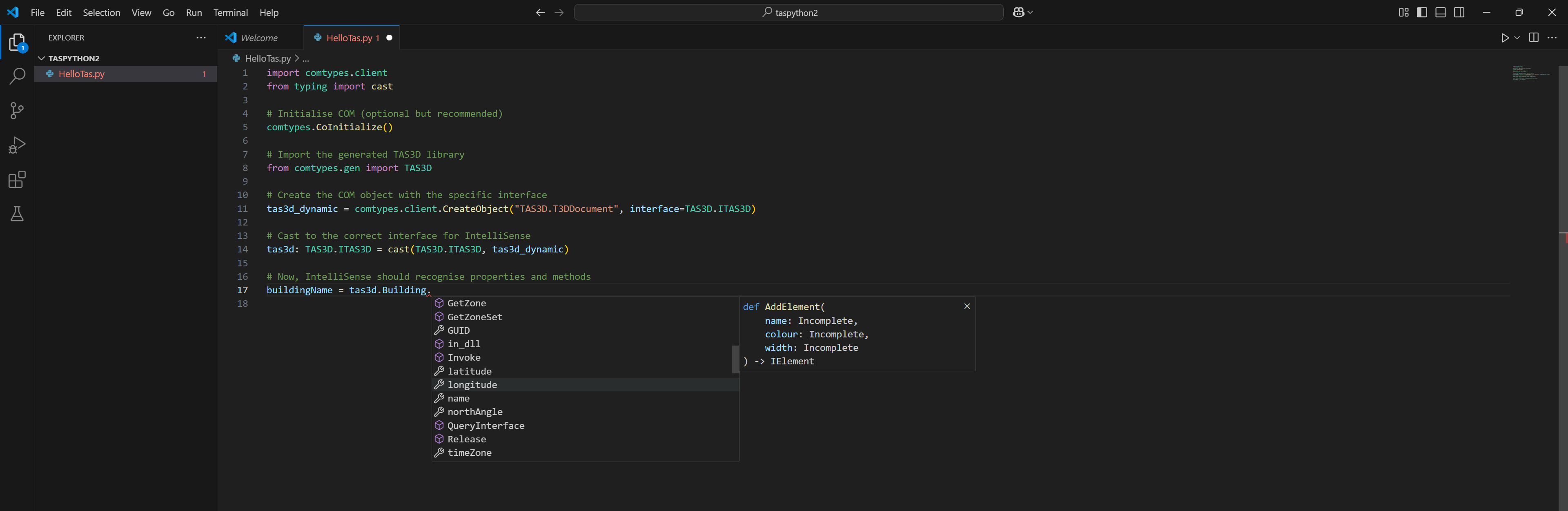
Screenshot of VSCode showing intellisense for python using the tas API.
A screenshot of a python IDE showing intellisense for the Tas type libaries.

Which tools should I use?

For this example, we will be using Python 3 in conjunction with Visual Studio Code as our IDE. You can also use Pycharm or Visual Studio, but I have chosen Visual Studio Code as it’s free and is relatively lightweight and requires minimal setup.

Step 1: Install Python

If you haven’t already installed Python, you can do so from python.org. I have installed Python version 3.13.1, but any version of Python 3 should work.

Step 2: Install Visual Studio Code

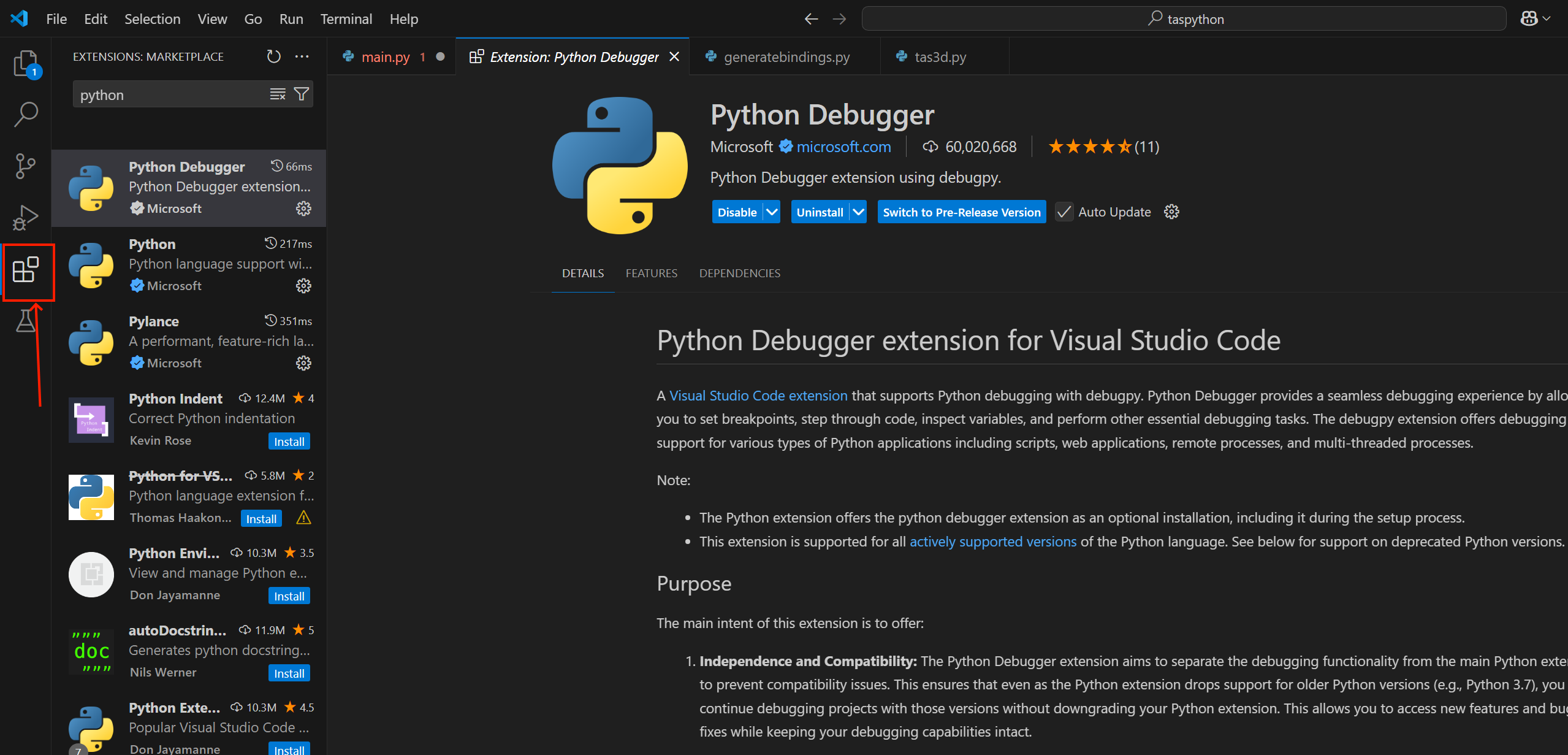
You can install Visual Studio Code from here. Once you have installed it, you’ll want to install the Python plugin. The first time you open a .py file in visual studio code, it will ask you if you want to install the Python plugin. Alternatively, you can just search from it in the online Extensions library/

Step 3: Install comtypes using pip

After you have installed Python, you’ll need to install the comtypes Python library. This library can be used to automatically create Python bindings for the Tas type libraries, which is how the Visual Studio Python interpreter learns about the Tas API. 

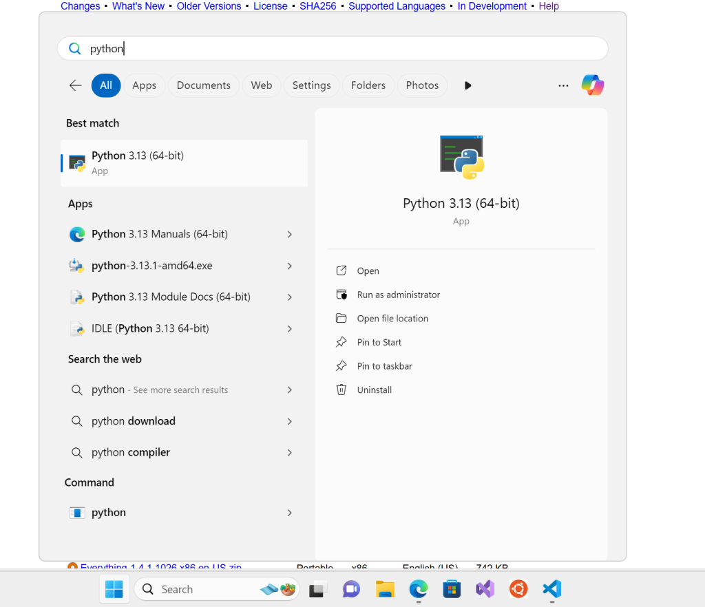
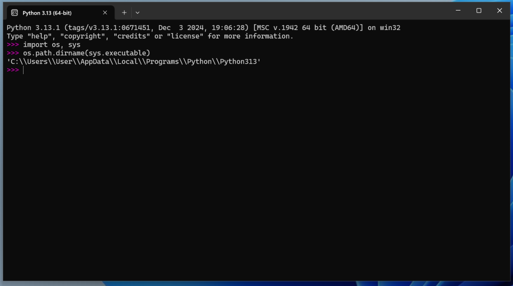
Open a python terminal by pressing the Start button and searching for Python:

With the Python shell open, enter the following code, pressing return after each statement, in order to determine where the Python executable is installed on your machine:

				
					import os, sys
os.path.dirname(sys.executable)


You should end up with something like the following:

We can see from the above that on my computer, Python is installed to C:\users\User\AppData\Local\Programs\Python\Python313. We will need to use this directory in order to install comtypes using pip.

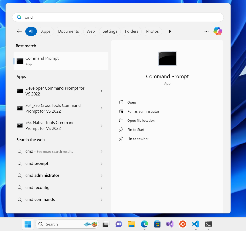
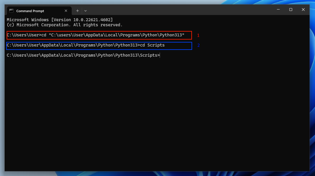
Open a command prompt and ‘change directory’ to the directory identified in the previous step:

Change directory using the cd command:

Change into the Scripts directory as per the above, and then you can run the pip install command in order to install comtypes:

				
					pip install comtypes


Step 4. Generate Bindings

Now we can use comtypes to generate bindings for the Tas type libraries. We will do this using a Python script which we should only have to run once, though it may need re-running from time to time if the bindings are stored in a temporary directory on your computer. Create a new file called GenerateBindings.py in visual studio code, and enter the following script:

				
					import os
import comtypes.client

# Define the directory containing the type libraries
type_lib_dir = r'C:\Program Files\Environmental Design Solutions Ltd\Tas'

# List of type library filenames
type_lib_files = ['TAS3D.tlb', 'tbd.tlb', 'tpd.tlb', 'twd.tlb', 'tai.tlb', 'tcr.tlb', 'tcd.tlb', 'tsd.tlb']

# Generate COM bindings for each type library
for tlb_file in type_lib_files:
    tlb_path = os.path.join(type_lib_dir, tlb_file)
    comtypes.client.GetModule(tlb_path)

print("COM bindings generated successfully for all type libraries.")


When you run this script, the bindings will be created immediately.

Step 5: Write a script to check it worked

Now we can write a script to check it worked. As a simple example, create a new file in visual studio code called HelloTas.py and enter the following:

				
					import comtypes.client
from typing import cast

# Initialise COM (optional but recommended)
comtypes.CoInitialize()

# Import the generated TAS3D library
from comtypes.gen import TAS3D  

# Create the COM object with the specific interface
tas3d_dynamic = comtypes.client.CreateObject("TAS3D.T3DDocument", interface=TAS3D.ITAS3D)

# Cast to the correct interface for IntelliSense
tas3d: TAS3D.ITAS3D = cast(TAS3D.ITAS3D, tas3d_dynamic)

# Now, IntelliSense should recognise properties and methods
buildingName = tas3d.Building.buildingName

#Print the building name to the console
print(buildingName)


You should notice that when you start entering the above, the Intellisense menu appears and gives you code suggestions:

Congratulations! You’re ready to write some Tas Python scripts. All of the scripts mentioned in the coding lesson blog posts so far can be converted to Python, so it might be a good idea to use these for inspiration when it comes to getting started!

CO₂ Generation Rates

Calculating Metabolic Pollutant Generation Rates (CO₂)

There are many regulations which endorse modelling occupant pollutant generation accumulation within buildings. For occupants, this pertains to carbon dioxide (CO2). Most standards set thresholds which should not be exceeded:

  • ASHRAE Standard 62.1
  • CIBSE Guide A
  • WELL Building Standard
  • LEED 
  • BREEAM 

Building simulation software often takes the CO2 generation rate as an input to the calculation, but modellers often are presented with a simple ‘number of occupants’ to base their assumptions on when it comes to occupancy gains and their pollutant generation rates. 

In this blog post, we’ll explore the relationship between ‘number of occupants’ and ‘CO2 generation rate’, and produce a basic calculator which can be used to aid calculating CO2 generation rates depending on the information you have available.

Why do our bodies produce CO2?

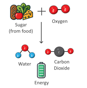
In order to convert food into energy, our bodies convert glucose and oxygen into energy, carbon dioxide and water. This process is known as respiration.

As most of us don’t just eat sugar (glucose), our bodies also have to convert things like proteins and carbohydrates into glucose at the start of the process. 

Converting different foods into glucose also requires energy, which is why metabolising different foods produces varying amounts of CO2. 

The equation for respiration is:

\( \text{C}_6\text{H}_{12}\text{O}_6 + 6 \, \text{O}_2 \rightarrow 6 \, \text{CO}_2 + 6 \, \text{H}_2\text{O} + \text{Energy (ATP)} \)

That is, glucose + oxygen -> carbon dioxide + water

sugar plus oxygen are used in respiration to produce water, carbon dioxide and metabolic energy.

What affects CO2 Generation Rates?

If you selected two random people from different age groups, genders and level of fitness and measured how much carbon dioxide these people expelled over the course of an hour, you would probably find that the amount of CO2 produced can vary quite significantly. This is because the amount of CO2 a person produces depends heavily on their diet and metabolism:

  • Metabolic Rate: This is the rate at which your body burns calories at rest. Higher metabolic rate = more CO2.
  • Physical activity level: When we exercise, we burn more calories and produce more CO2.
  • Diet: Different food gets metabolised into different amounts of CO2 due to different metabolic pathways. Eating more protein can produce more CO2 compared to carbohydrates. 
  • Body size & composition: An increase in body weight is usually associated with a higher metabolic rate
  • Age and gender: Metabolic rate usually declines with age. Men tend to have higher metabolic rates than women.
  • Environmental factors: Temperature and altitude can affect how our body produces energy (and CO2 as a biproduct).
  • Health conditions: e.g. hyperthyroidism can increase metabolic rate and therefore CO2 production.

Respiratory Quotient (RQ)

From the respiration equation mentioned earlier, we can see that the amount of CO2 a person produces is directly related to how much oxygen they consume during respiration.

The ratio of CO2 relesed to O2 consumed is known as the Respiratory Quotient (RQ):

\( \text{RQ} = \frac{\text{Volume of } \text{CO}_2 \, \text{produced}}{\text{Volume of } \text{O}_2 \, \text{consumed}} \)

We mentioned earlier that different foods are converted to glucose in order for respiration to take place. As this conversion, known as gluconeogenesis, relies on energy to take place, this implies that different foods consumed result in different amounts of CO2 being produced during metabolism. Therefore, the RQ varies depending on diet, and some example figures are given in the tables below.

Converting number of people to CO2 generation rates

In order to derive a relation between the number of people in a space and the amount of CO2 produced by each person per hour, we will use the following relation:

“For every 1 litre of oxygen the body uses, approximately 5 calories are expended”

Calories are a measure of how much energy we can consume during respiration, so therefore if we calculate how much oxygen a person consumes, we can use the Respiratory Quotient to determine how much CO2 is produced as a biproduct. 

We can relate kcals to Joules with the following relation:

  • \( 1 \, \text{kcal} = 4184 \, \text{Joules (J)} \)

And Watts, which we often use in building simulation software as an input, are related to joules by:

  • \( 1 \, \text{Watt (W)} = 1 \, \frac{\text{Joule (J)}}{\text{Second (s)}} \)

Putting these relations together, we can deduce:

  • \( 1 \, \text{litre O}_2/\text{min} \times 5 \, \text{kcal}/\text{litre O}_2 \times 4184 \, \text{J}/\text{kcal} = 20920 \, \text{J}/\text{min} \)

Converting to Joules per second (Watts):

  • \( \frac{20920 \, \text{J}/\text{min}}{60 \, \text{sec}/\text{min}} = 348.67 \, \text{J}/\text{sec} = 348.67 \, \text{Watts} \)

For 1 ml O2/ minute:

\( \frac{348.67 \, \text{Watts}}{1000 \, \text{ml}/\text{litre}} = 0.34867 \, \text{Watts}/\text{ml}/\text{O}_2/\text{min} \)

So therefore:

\( \text{Metabolic Rate (W)} = \text{VO}_2 \, (\text{ml}/\text{min}) \times 0.34867 \)

Rearranging so that we can calculate VO2:

\( \text{VO}_2 \, (\text{ml}/\text{min}) = \frac{\text{Metabolic Rate (W)}}{0.34867} \)

And converting to CO2 by multiplying by the Respiratory Quotient (RQ):

\( \text{CO}_2 \, (\text{ml}/\text{min}) = \frac{\text{Metabolic Rate (W)}}{0.34867} \times \text{RQ} \)

Converting to litres/hour:

\( \text{CO}_2 \, (\text{L}/\text{hour}) = \left( \frac{\text{Metabolic Rate (W)}}{0.34867} \right) \times \text{RQ} \times \frac{60}{1000} \)

Example Metabolic Rates

This table lists some rate of heat emissions for mixtures of males/females. 

Degree of Activity Typical Building Total Rate of Heat Emission (W) Sensible Heat (W) Latent Heat (W)
Seated at theatre Theatre, cinema (matinee) 95 65 30
Seated at theatre, night Theatre, cinema (night) 105 70 35
Seated, very light work Offices, hotels, apartments 115 70 45
Moderate office work Offices, hotels, apartments 130 75 55
Standing, light work; walking Department store, retail store 130 75 55
Walking; standing Bank 145 75 70
Sedentary work Restaurant 160 80 80
Light bench work Factory 220 80 140
Moderate dancing Dance hall 250 90 160
Walking; light machine work Factory 295 110 185
Bowling Bowling alley 425 170 255
Heavy work Factory 425 170 255
Heavy machine work; lifting Factory 470 185 285
Athletics Gymnasium 525 210 315

Source: ASHRAE Handbook: Fundamentals (2001)

Example Respiratory Quotients (RQ)

Substrate Respiratory Quotient (RQ)
Carbohydrate 1.00
Fat 0.696
Protein 0.818
Non Dairy 0.86
Mixed Diet 0.8

Source: Exercise Physiology. Nutrition, Energy, and Human Performance by William D. McArdle, Frank I. Katch, Victor L. Katch  & Wikipedia 

Putting it all together: Example

Let’s calculate the CO2 pollutant generation rate for an office with 1 occupant and a floor area of 3m2. Assumptions:

  • Metabolic rate 130W (Moderate office work)
  • Mixed diet (RQ = 0.8)
The calculation is therefore:
 
\( \text{CO}_2 \, (\text{L}/\text{hour}) = \left( \frac{130}{0.34867} \right) \times 0.8 \times \frac{60}{1000} = 17.897 \)
 
And to convert to litres / hour / m2, divide by the floor area:
 
\( \text{CO}_2 \, (\text{L}/\text{hour}/\text{m}^2) = \frac{\text{CO}_2 \, (\text{L}/\text{hour})}{\text{Area} \, (\text{m}^2)} = \frac{178.97}{3} = 5.97 \, \text{L}/\text{hour}/\text{m}^2 \)

Carbon Dioxide Calculator

To save time, you can use the following handy carbon dioxide pollutant generate calculator to help calculate pollutant generation rates for use in Tas:

This calculator uses the methods discussed above to equate number of occupants to CO2 pollutant generation rates. If you would like us to add more activity levels to this calculator, please get in touch. As metabolic rates vary so significantly between individuals, we would always recommend performing sensitivity analysis to ensure your buildings perform well given the inherent uncertainty in the pollutant generation rates. 

Other useful conversions

In building simulation software, we often work with Watts as our primary unit for metabolic rates as these directly relate to the amount of sensible and latent heat gain occupants emit into a space. In other industries, however, it is quite common to work with METs.

What is a MET?

1 MET is the rate of energy expenditure at rest, approximately equal to 1 kcal per kg of body weight per hour, or 3.5 mL of oxygen consumed per kg of body weight per minute

Converting METs to Watts

Converting METs to Watts is fairly straightforward if you know the body weight of the individual:

\( \text{Watts (W)} = \text{MET} \times \text{Body Weight (kg)} \times 1.225 \)

Converting Watts/m2 to Watts

Sometimes heat generation rates for a given activity are specified in terms of W/m2, so therefore they need to be multiplied by the surface area of a human body. The average surface area of an adult human body is 1.8m2, so this may be helpful if you are using Table 1.4 from CIBSE guide A. 

Body Weight (kg) Surface Area (m²)
1 0.10
2 0.16
4 0.26
6 0.34
8 0.42
10 0.49
15 0.65
20 0.79
25 0.92
30 1.10
35 1.20
40 1.30
Table of body surface area in children, taken from nice.org.uk

Calculating CO2 generation for different age groups

To calculate CO2 generation rates for different age groups, first look up the average body weight by expected age of the occupant in the following table:

Age Range Average Weight (kg)
0-6 months 3.3 - 7.5
1-2 years 7.9 - 9.2
2-4 years 12 - 15
8-10 years 19.5 - 25.5
14-16 years 45 - 53
18-20 years 56 - 58

Next, look up the average surface area from the body weight vs surface area table above. Or, for an adult male, assume 1.8m2 as per CIBSE guide. 

Then, look up the heat generation rate per unit area of body from the following table:

Activity Heat Generation (W/m²)
Resting
Sleeping 41
Reclining 46
Seated, Quiet 58
Standing, Relaxed 70
Walking (Level)
0.9 m/s 116
1.3 m/s 151
1.8 m/s 221
Office Work
Reading, Seated 58
Writing 58
Typing 64
Filing, Seated 70
Filing, Standing 81
Lifting/Packaging 122
Occupational
Cooking 81-134
House Cleaning 99-198
Seated, Heavy Limb Movement 128
Machine Sawing 105
Light Machine Work 93-116
Heavy Machine Work 175
Handling 50 kg Bags 233
Leisure
Dancing 82-256
Tennis 210-233
Basketball 294-442
Wrestling 407-506

Figures for this table were taken from CIBSE guide A 2006, Table 1.4

Multiply the average surface area by the Heat Generation from the table above to get a metabolic rate in Watts, which you can then enter into the calculator above by selecting the Other option. 

Coincidental Loads

Understanding Load Calculations in Building Simulation: Coincidental Loads vs. Steady-State Loads

In the world of building design and simulation, accurately calculating loads is essential for ensuring optimal performance and energy efficiency. As buildings evolve to meet the demands of modern life, understanding the nuances of different load types becomes increasingly critical. Among these, coincidental loads and steady-state loads play pivotal roles in how we design systems that can adapt to varying conditions.

In Tas, loads can be calculated using Heating & Cooling Design Days via the Design Day Wizard, or directly from the Dynamic Simulation Results. In this blog post, we will explore the difference between the two methods and how this relates to coincidental and steady state loads. 

Steady-State vs Dynamic Loads

Before we discuss what coincidental loads are, we need to discuss the difference between steady-state and dynamic loads. 

Steady-state loads are characterised by their predictability and consistency over time. For instance, the Chartered Institution of Building Services Engineers (CIBSE) employs steady-state heating design day calculations to establish the heating requirements of a building. 

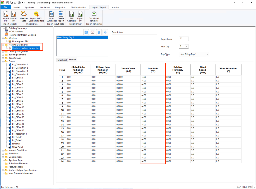
These calculations assume constant conditions for each hour of the design day, including factors such as indoor temperature, occupancy, and weather patterns. A fixed external dry bulb temperature is selected, usually -4°C in the UK, and solar , occupancy and equipment gains are removed. As the hourly conditions do not change from hour to hour, they are considered to be steady and therefore simulating this day over and over should eventually cause the results to converge. 


For Heating Design Days, a fixed external dry bulb temperature of -4°C is typically used for sizing in the UK. Other internal gains are removed, such as solar gain and occupancy/equipment gains.

The Design Day Wizard simplifies this process, allowing you to set up these calculations efficiently.

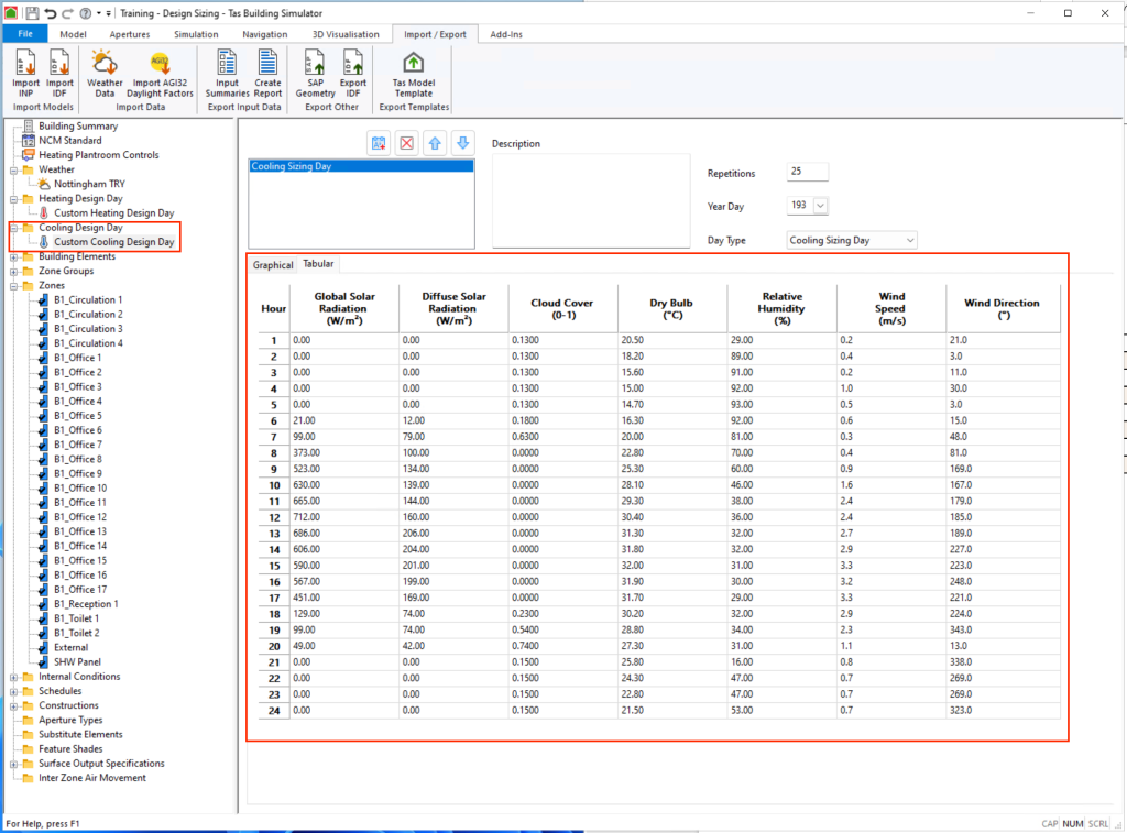
Similarly, the Design Day Wizard can also be utilised for cyclic cooling design day calculations, which differ slightly in that the same day of weather is simulated repeatedly but the weather does typically vary throughout the day:


Typically, a hot day of weather is picked for a cooling design day and this day is simulated repeatedly. Other heat gains are usually included, such as occupancy and equipment gains.

Advantages of Steady-State Loads:

  • Simplicity: Steady-state calculations are relatively straightforward and easy to implement, making them accessible for designers.
  • Consistency: They provide reliable estimates for typical operating conditions, allowing for easier compliance with regulations and standards.
  • Time Efficiency: The use of tools like the Design Day Wizard streamlines the process.

Disadvantages of Steady-State Loads:

  • Oversizing Risk: These calculations often lead to oversizing of systems since they focus on worst-case scenarios or peak demands that may not occur simultaneously. As a result, systems may be designed to handle maximum loads that are infrequent or unlikely.
  • Lack of Flexibility: Steady-state calculations do not account for fluctuations in usage or environmental conditions, which can lead to inefficiencies and higher operational costs.
  • Limited Realism: By neglecting the dynamic nature of actual building usage, steady-state calculations may not accurately reflect how systems will perform under varying conditions, potentially resulting in increased energy consumption.

In contrast, dynamic loads fluctuate in response to varying conditions and usage patterns, leading to the concept of coincidental loads. 

What are Coincidental Loads?

Imagine you are simulating a building with 5 zones. These zones are called Zone A, Zone B, Zone C etc. You simulate the entire year, and have results for every hour of the year for these zones…

One way of determining the Peak Load for these zones would be to find the maximum value in each column and sum them:

Office Zone Individual Peak Heating Load (W) Peak Occurrence Time
Zone A 10,000 Day 1, 9:00 AM
Zone B 8,000 Day 5, 9:00 AM
Zone C 12,000 Day 5, 10:00 AM
Zone D 6,000 Day 12, 11:00 AM
Zone E 5,000 Day 11, 2:00 PM
Total Individual Peak 41,000

The total individual peak loads for each office zone represent the maximum heating demand that each zone can reach. However, these peaks may not occur simultaneously; they could happen on different days and at different times.

As a result, the peak load that an HVAC system needs to accommodate when conditioning these spaces is not simply the sum of the individual peak loads. Instead, the actual peak load for the HVAC system corresponds to the specific day and hour when the combined loads of all zones are at their highest.

This is known as a coincidental load, which represents the maximum demand that the HVAC system must be prepared to meet when all zones reach their peak demand at the same time. 

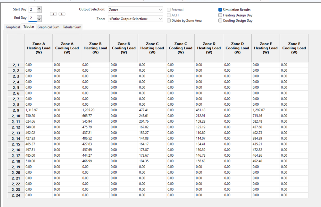
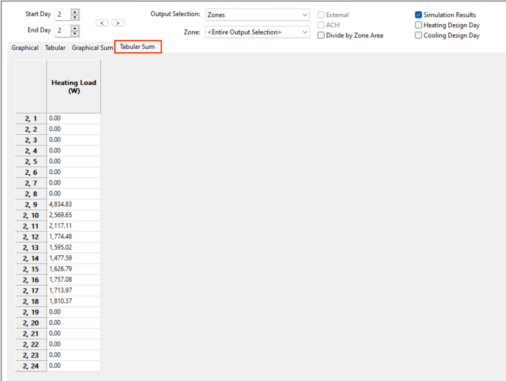
Hour Zone A Heating Load (W) Zone B Heating Load (W) Zone C Heating Load (W) Zone D Heating Load (W) Zone E Heating Load (W) Total Heating Load (W)
2, 9 1,313.97 1,285.20 477.41 461.18 1,297.07 4,834.83
2, 10 730.20 665.77 245.61 212.91 715.16 2,578.65
2, 11 624.66 545.94 204.76 159.28 582.48 2,116.12
2, 12 548.08 475.79 167.82 125.19 457.60 1,774.48
2, 13 492.02 437.21 152.27 110.80 402.73 1,595.03
2, 14 427.83 406.52 144.88 114.07 384.29 1,477.59
2, 15 465.37 427.63 164.17 134.41 435.21 1,826.99

So, to be clear, the coincidental load is found by summing the rows and finding the maximum value in the Total Heating Load column throughout the year. 

In Tas, this is easily achieved in the results viewer by using the Tabular Sum table:

Coincidental Loads & Design Days

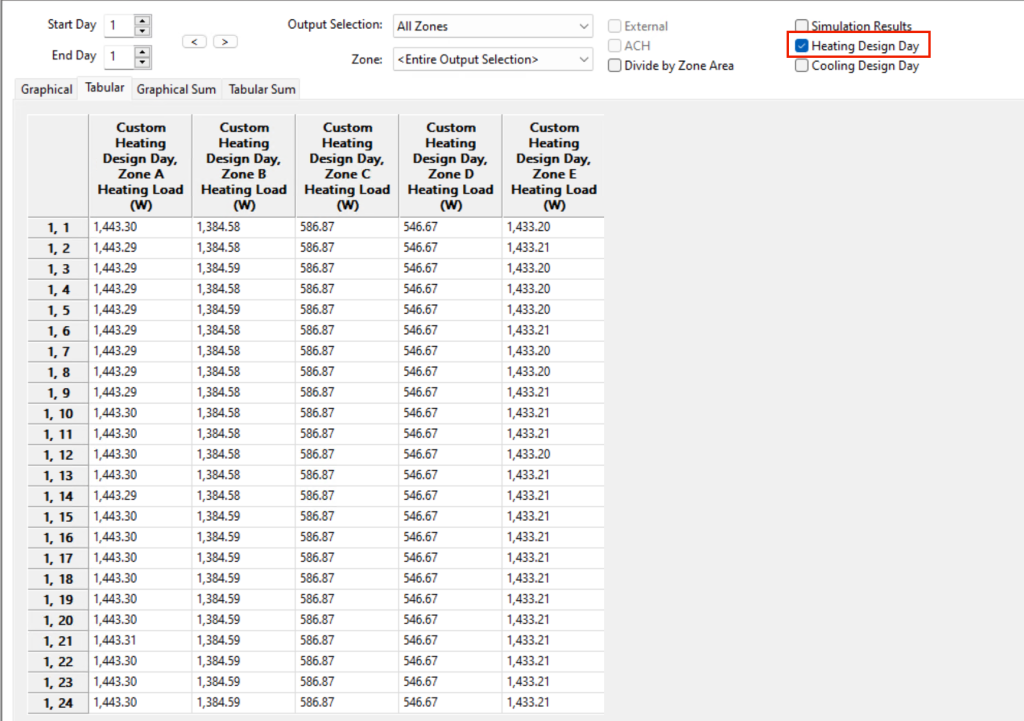
Heating Design Days produce a steady state result; the result converges, so the simulation results are the same for each hour:

As the results are the same for every hour, the coincidental peak is the same as the sum of the individual peaks due to the nature of the calculation.

With cyclic cooling design days, the results may vary hour to hour so it is possible that the coincidental load may be different to the sum of the individual peaks:

Hour Zone A (W) Zone B (W) Zone C (W) Zone D (W) Zone E (W) Coincidental (W)
193, 1 0 0 0 0 0 0
193, 2 0 0 0 0 0 0
193, 3 0 0 0 0 0 0
193, 4 0 0 0 0 0 0
193, 5 0 0 0 0 0 0
193, 6 0 0 0 0 0 0
193, 7 0 0 0 0 0 0
193, 8 0 0 0 0 0 0
193, 9 0 0 0 0 32.42 32.42
193, 10 744.19 806.96 329.64 366.47 804.12 3051.38
193, 11 817.84 877.64 359.59 395.19 896.80 3347.06
193, 12 878.05 936.04 385.12 420.38 971.08 3590.67
193, 13 917.72 976.72 403.29 440.83 1,005.45 3744.01
193, 14 975.07 1,011.81 430.39 452.72 1,047.70 3917.69
193, 15 1,026.89 1,032.86 458.94 458.89 1,083.71 4061.29
193, 16 1,067.16 1,039.12 486.24 459.08 1,107.94 4159.54
193, 17 1,099.06 1,043.97 501.24 456.24 1,128.63 4229.14
193, 18 1,020.67 995.22 434.54 423.60 1,044.74 3918.77
193, 19 0 0 0 0 0 0
193, 20 0 0 0 0 0 0
193, 21 0 0 0 0 0 0
193, 22 0 0 0 0 0 0
193, 23 0 0 0 0 0 0
193, 24 0 0 0 0 0 0

In this case, the sum of the individual peaks (4231.98W) is slightly larger than the coincidental peak (4,229.14W).  If the peak for zone D occurred at hour 17 as with the other zones, the coincidental peak would be equal to the sum of the individual peaks. 

Finding Coincidental Peaks in Tas

The method you use to obtain coincidental loads from Tas depends if you are using design days or the dynamic simulation. 

Design Days

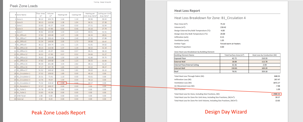
If your design day is steady state, i.e. the results are not varying hour by hour, the coincidental load is equal to the peak load so the results from the design day wizard and the peak zone loads report can be used directly. They will be equal. 

If your design day is cyclic as is often the case with cooling design days, you can obtain the coincidental peak by looking at the tabular sum results in the TSD file and finding the maximum value.

Dynamic Simulation

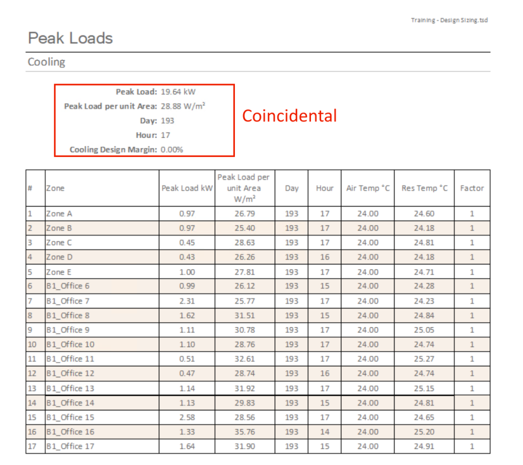
If you are obtaining loads from the dynamic simulation, the Peak Loads report will report the coincidental peak in addition to the individual peaks, for the zones included in the report. 

You can also obtain the coincidental peak from the dynamic simulation by looking at the tabular sum in the TSD results and finding the peak. 

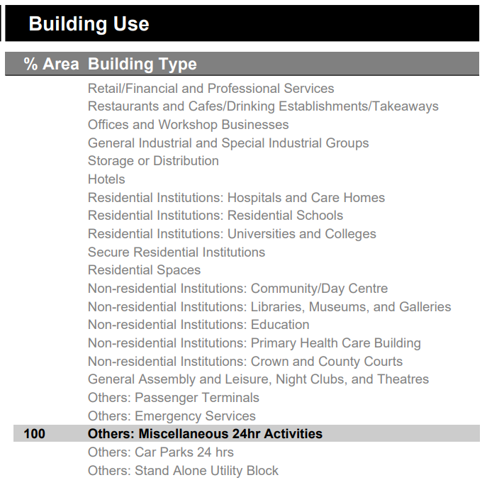
Part L 2021 Building Use Types

Part L 2021 Building Use Types

Sometimes it’s not always clear which NCM internal conditions correspond to each of the Building Use Types listed in the BRUKL document. This table lists them all out, clearly. 


These categories are the categories assigned by the BRUKL generator version 6.1.4.0, in conjunction with the 6.1.b internal conditions. 

Retail/Financial and Professional Services

  • A1A2_CarPark
  • A1A2_Circulation
  • A1A2_DepStoreSales
  • A1A2_DepStoreSalesChill
  • A1A2_DepStoreSalesElectric
  • A1A2_Display
  • A1A2_EatDrink
  • A1A2_FoodPrep
  • A1A2_Laund
  • A1A2_Office
  • A1A2_Plant
  • A1A2_RetWareSales
  • A1A2_RetWareSalesChill
  • A1A2_RetWareSalesElectric
  • A1A2_Sales
  • A1A2_SalesChill
  • A1A2_SalesElectric
  • A1A2_Store
  • A1A2_Toilet

Restaurants and Cafes/Drinking Establishments/Takeaways

  • A345_Circulation
  • A345_EatDrink
  • A345_FoodPrep
  • A345_Office
  • A345_Plant
  • A345_Stage
  • A345_Store
  • A345_Toilet

Offices and Workshop Businesses

  • B1_CarPark
  • B1_Changing
  • B1_Circulation
  • B1_EatDrink
  • B1_FoodPrep
  • B1_Gym
  • B1_Office
  • B1_Plant
  • B1_Reception
  • B1_Store
  • B1_Toilet
  • B1_WkshpSS

Hotels

  • C1_Bath
  • C1_Bedroom
  • C1_Changing
  • C1_Circulation
  • C1_DrySptHall
  • C1_EatDrink
  • C1_EnsuiteBedroom
  • C1_FitGym
  • C1_FoodPrep
  • C1_Laund
  • C1_Office
  • C1_Plant
  • C1_Reception
  • C1_Store
  • C1_Toilet

Residential Institutions: Residential Schools

  • C2_Schools_Bath
  • C2_Schools_Bedroom
  • C2_Schools_Changing
  • C2_Schools_Circulation
  • C2_Schools_CommunalArea
  • C2_Schools_DrySptHall
  • C2_Schools_EatDrink
  • C2_Schools_FoodPrep
  • C2_Schools_HighDensIT
  • C2_Schools_Lab
  • C2_Schools_Laund
  • C2_Schools_Lecture
  • C2_Schools_Office
  • C2_Schools_Plant
  • C2_Schools_Reception
  • C2_Schools_Store
  • C2_Schools_Teaching
  • C2_Schools_Toilet
  • C2_Schools_WkshpSS

Residential Institutions: Universities and Colleges

  • C2_Uni_Bath
  • C2_Uni_Bed
  • C2_Uni_Changing
  • C2_Uni_Circulation
  • C2_Uni_CommunalArea
  • C2_Uni_DrySptHall
  • C2_Uni_EatDrink
  • C2_Uni_FitGym
  • C2_Uni_FoodPrep
  • C2_Uni_HighDensIT
  • C2_Uni_Lab
  • C2_Uni_Laund
  • C2_Uni_Lecture
  • C2_Uni_Office
  • C2_Uni_Plant
  • C2_Uni_Reception
  • C2_Uni_Store
  • C2_Uni_Tea
  • C2_Uni_Toilet
  • C2_Uni_WkshpSS

Others: Car Parks 24 hrs

  • CarPark_CarPark
  • CarPark_Circulation
  • CarPark_Office
  • CarPark_Plant
  • CarPark_Toilet

Non-residential Institutions: Crown and County Courts

  • Court_Cell
  • Court_Circulation
  • Court_EatDrink
  • Court_FoodPrep
  • Court_Lecture
  • Court_Office
  • Court_Plant
  • Court_Reception
  • Court_Store
  • Court_Toilet

Non-residential Institutions: Education

  • D1_Edu_Changing
  • D1_Edu_Circulation
  • D1_Edu_DrySptHall
  • D1_Edu_EatDrink
  • D1_Edu_FoodPrep
  • D1_Edu_HighDensIT
  • D1_Edu_Lab
  • D1_Edu_Lecture
  • D1_Edu_Office
  • D1_Edu_Plant
  • D1_Edu_Reception
  • D1_Edu_Store
  • D1_Edu_Teaching
  • D1_Edu_Toilet
  • D1_Edu_WkshpSS

General Assembly and Leisure, Night Clubs, and Theatres

  • D2_Auditoria
  • D2_Changing_High
  • D2_Changing_Low
  • D2_Changing_Medium
  • D2_Circulation
  • D2_CirculationPub
  • D2_DrySptHall
  • D2_EatDrink
  • D2_FitGym
  • D2_FitStud
  • D2_IceRink
  • D2_Laund
  • D2_Lecture
  • D2_Office
  • D2_Plant
  • D2_Reception
  • D2_Sales
  • D2_Stage
  • D2_Store
  • D2_Toilet
  • D2_WkshpSS

Non-residential Institutions: Community/Day Centre

  • DayCtr_Changing
  • DayCtr_Circulation
  • DayCtr_DrySptHall
  • DayCtr_EatDrink
  • DayCtr_FoodPrep
  • DayCtr_Lecture
  • DayCtr_Office
  • DayCtr_Plant
  • DayCtr_Reception
  • DayCtr_Store
  • DayCtr_Toilet
  • DayCtr_WkshpSS

Residential Spaces

  • Dwell_DomBath
  • Dwell_DomCirculation
  • Dwell_DomCommonAreas
  • Dwell_DomDining
  • Dwell_DomKitchen
  • Dwell_DomLounge
  • Dwell_DomToilet

Others: Emergency Services

  • EmgcySvc_Bath
  • EmgcySvc_Bed
  • EmgcySvc_Cell
  • EmgcySvc_Circulation
  • EmgcySvc_DrySptHall
  • EmgcySvc_EatDrink
  • EmgcySvc_FitGym
  • EmgcySvc_FoodPrep
  • EmgcySvc_Office
  • EmgcySvc_Plant
  • EmgcySvc_Reception
  • EmgcySvc_Store
  • EmgcySvc_Toilet

Residential Institutions: Hospitals and Care Homes

  • Hosp_AECons
  • Hosp_Bath
  • Hosp_Bed
  • Hosp_Bed_24x7
  • Hosp_Changing
  • Hosp_Circulation
  • Hosp_CirculationPub
  • Hosp_ClassRm
  • Hosp_Diagnostic
  • Hosp_EatDrink
  • Hosp_FoodPrep
  • Hosp_IndProcess
  • Hosp_Lab
  • Hosp_Laund
  • Hosp_Lecture
  • Hosp_Office
  • Hosp_OpTheatre
  • Hosp_Physiotherapy
  • Hosp_Plant
  • Hosp_PostMortem
  • Hosp_Reception
  • Hosp_Store
  • Hosp_Toilet
  • Hosp_Wards

General Industrial and Special Industrial Groups

  • Indust_Circulation
  • Indust_EatDrink
  • Indust_FoodPrep
  • Indust_IndProcess
  • Indust_Lab
  • Indust_Office
  • Indust_Plant
  • Indust_Reception
  • Indust_Store
  • Indust_Toilet
  • Indust_WareStore

Non-residential Institutions: Libraries, Museums, and Galleries

  • LibMusGall_Circulation
  • LibMusGall_DisplayPublic
  • LibMusGall_EatDrink
  • LibMusGall_FoodPrep
  • LibMusGall_Lab
  • LibMusGall_Lecture
  • LibMusGall_Office
  • LibMusGall_Plant
  • LibMusGall_Reception
  • LibMusGall_Store
  • LibMusGall_Toilet
  • LibMusGall_WkshpSS

Others: Miscellaneous 24hr Activities

  • Misc24Hr_DataCentre
  • Misc24Hr_HeavyPlant
  • Misc24Hr_ServerRoom
  • Misc_24x7Office
  • Misc_24x7Toilet

Secure Residential Institutions

  • Prison_Bath
  • Prison_Cell
  • Prison_Changing
  • Prison_Circulation
  • Prison_ClassRm
  • Prison_DrySptHall
  • Prison_EatDrink
  • Prison_FitGym
  • Prison_FoodPrep
  • Prison_Laund
  • Prison_Lecture
  • Prison_Office
  • Prison_Plant
  • Prison_Reception
  • Prison_Store
  • Prison_Toilet
  • Prison_WkshpSS

Non-residential Institutions: Primary Health Care Building

  • PrmHlthCare_Circulation
  • PrmHlthCare_Office
  • PrmHlthCare_Plant
  • PrmHlthCare_Reception
  • PrmHlthCare_Store
  • PrmHlthCare_Toilet

Others: Stand Alone Utility Block

  • Stand_Changing_High
  • Stand_Changing_Low
  • Stand_Changing_Medium

Others: Passenger Terminals

  • Terminals_Checkin
  • Terminals_Office
  • Terminal_Circulation
  • Terminal_EatDrink
  • Terminal_FoodPrep
  • Terminal_Lounges
  • Terminal_Plant
  • Terminal_Reception
  • Terminal_Store
  • Terminal_Toilet
  • Terminal_WaitRm

Storage or Distribution

  • Ware_24x7Office
  • Ware_24x7WareStore
  • Ware_Changing
  • Ware_Circulation
  • Ware_EatDrink
  • Ware_FoodPrep
  • Ware_Office
  • Ware_Plant
  • Ware_Reception
  • Ware_Store
  • Ware_Toilet
  • Ware_WareStore

Rhino to Tas: How to with Honeybee

Creating Tas models with Rhino & Honeybee

Rhinoceros, otherwise known as Rhino3D, is a freeform surface modeller that is gaining popularity amongst energy modellers and architects for its ease of use in creating complex geometries. Not only that, but Rhino has a diverse range of plugins which make it possible to perform building energy analysis using interoperability with simulation engines such as Tas. In this blog post, we’ll walk through using the Honeybee plugin by Ladybug tools to link Rhino and Tas. 

What are Grasshopper, Ladybug Tools & Honeybee?

Ladybug tools is a collection of applications that support environmental design founded in 2012. These applications are opensource, and are free to use. 

One of these tools is called Honeybee, and this tool is a plugin for Grasshopper, a parametric modelling tool which is part of Rhino. 

Honeybee can be used to perform daylight simulations using Radiance, and simulate energy models using OpenStudio and EnergyPlus. Honeybee can also be used to produce IDF and gbXML files, both of which provide a route into Tas. 

gbXML? IDF? What's the difference?

Both gbXML and IDF are industry standard formats that are designed to allow building design software to share and communicate data. Whilst most building design packages can export gbXML, very few produce gbXML files that contain more than just geometry.

Fortunately, IDF files often contain both geometry and the data required to perform a full building simulation. IDF files produced using Honeybee contain geometry, internal conditions, construction information, design conditions and more, so we recommend using IDF files unless you’re only interested in importing Rhino geometry into Tas. 

How do I get started?

In order to get started with Rhino and Honeybee, you’ll first need to download and install Rhino. At the time of writing, you can get an 90 day trial if you do not have a license. 

Next, you’ll need to download and install Ladybug tools from Food4Rhino. This is a zip file, so unzip it and start Rhino. Then launch Grasshopper, and open the installer.gh file within Grasshopper:


After running the installation script and restarting Rhino, you should see the Ladybug tools appear in Grasshopper.

Note that you will also need to install OpenStudio if you want to generate IDF files. 

Creating Rhino Geometry

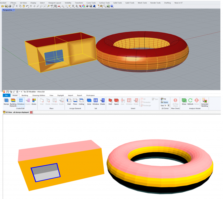
Now we’re ready to create some simple geometry in Rhino, to get ready for export. Let’s start by drawing a two zone model with a couple of windows – this way we can check that our adiabatic links are created correctly, and we’ll be able to see the principles behind marking surfaces as windows. Note that there are several ways to achieve the same outcome in Rhino, so feel free to experiment!

In the video below, I demonstrate how to:

  • Set the Rhino units
  • Draw two connected cuboids
  • Draw surfaces where the windows will be

It is important to remember that two touching faces must have the same dimensions in order to form an adiabatic link when using Honeybee. 

Setting up Honeybee in Grasshopper

Now that we’ve installed Honeybee and created some geometry in Rhino, we can start setting up our Grasshopper document. In the below video, I demonstrate how to produce a gbXML and an IDF file. I also demonstrate how to modify one of the Honeybee components to produce the IDF file without simulating the OpenStudio project..which saves a lot of time!

To skip running the open studio project and copy the IDF file to a directory of our choice, we can find the line containing run_idf and comment it out using a # at the start of the line. 

				
					import shutil
        elif run_ in (1, 3):  # run the resulting idf throught EnergyPlus
            shutil.copyfile(idf,_idfPathOut)
            #sql, zsz, rdd, html, err = run_idf(idf, _epw_file, silent=silent)

    # parse the error log and report any warnings
#    if run_ in (1, 3) and err is not None:
#        err_obj = Err(err)
#        print(err_obj.file_contents)
#        for warn in err_obj.severe_errors:
#            give_warning(ghenv.Component, warn)
#        for error in err_obj.fatal_errors:
#            raise Exception(error)


We have also used shutil.copyfile to copy the IDF file to the path of our choosing using the _idfPathOut parameter we added to the ModelToOSM component. For full details, see the video above.

Commenting out the end of the script stops any error messages appearing when we attempt to run the component. 

Importing the IDF into Tas

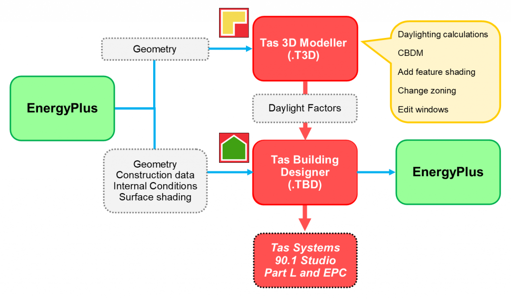
Once we’ve created our IDF file, we can import it into Tas using the IDF tool. We can optionally create a Tas3D model for shading calculations, import constructions & geometry and even specify the weather we want to use to simulate. In other words, the model is ready to go!

Rhino to Tas Workflow Summary

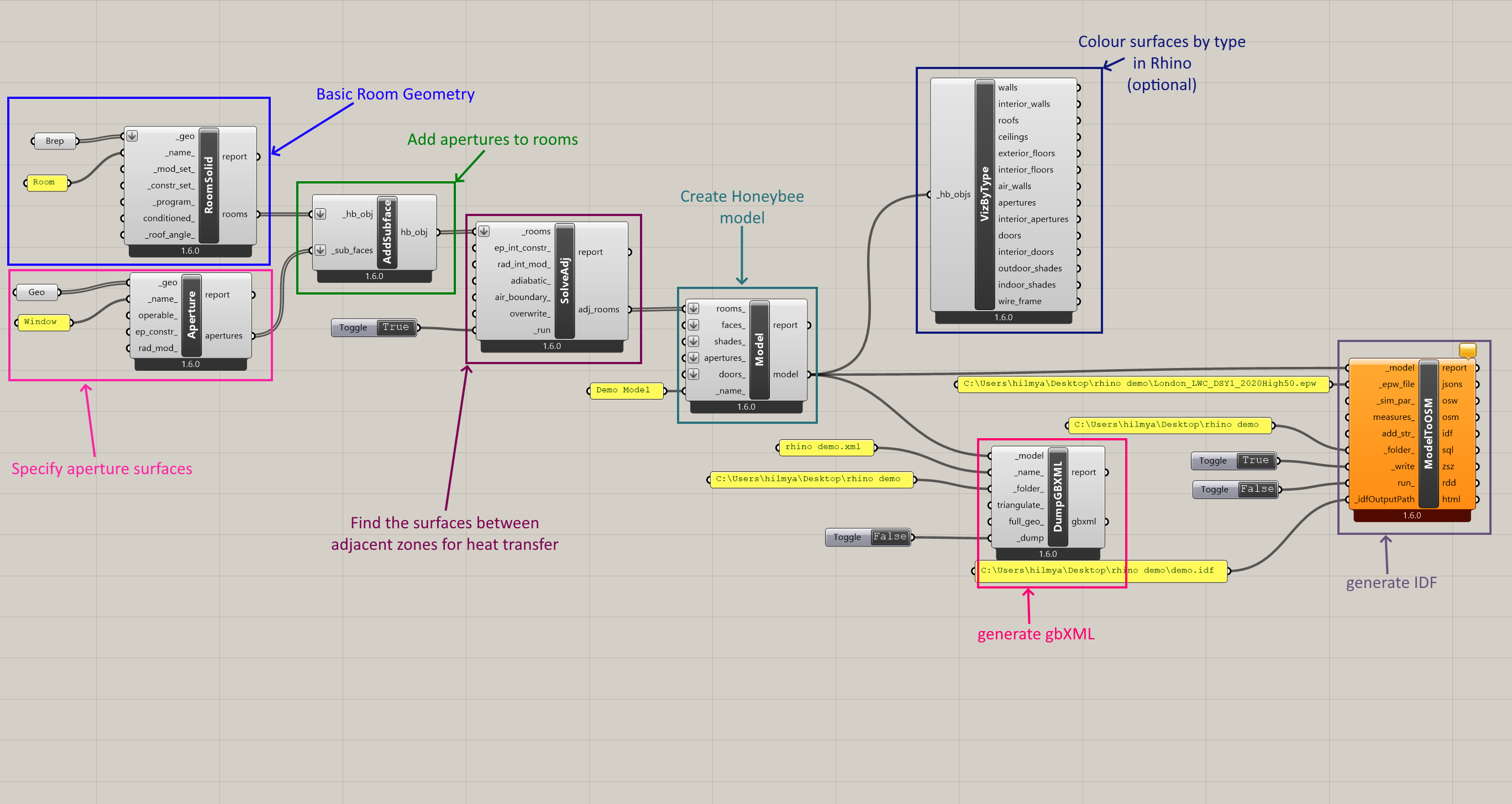
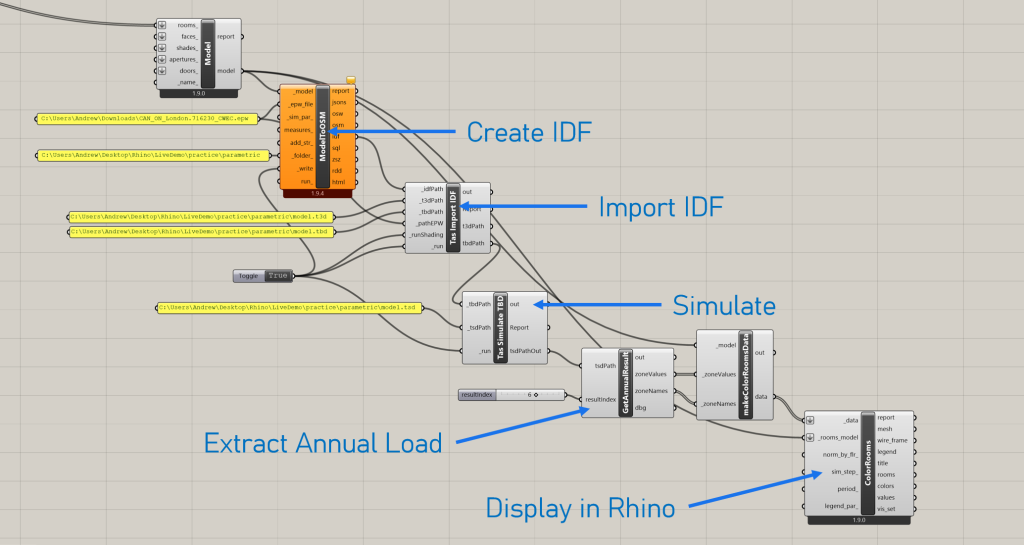
Below is a labelled Grasshopper diagram showing the key steps in creating gbXML and IDF files from Rhino. Remember, this is just one way to do it! Some of the components can be linked together in a different order, and some can be omitted. If you wanted to model % glazing, for example, you could add the apertures straight to the HoneyBee model and skip specifying and combining them. 

As the Rhino files are saved separately to the Grasshopper files, you can save the Grasshopper files and re-use them on future projects just by updating the geometry components each time. 

What else is Possible with Tas & Rhino?

As Grasshopper provides a visual programming interface to Rhino and Tas has a programming interface, the two can be linked to achieve endless outcomes – from parametric runs to performing full energy simulations and visualising the results in Rhino. 

You can create your own Tas Grasshopper code modules via python scripts:

				
					import win32com.client

#open the building simulator and then open a file
tbdDoc = win32com.client.Dispatch("TBD.Document")
tbdDoc.openReadOnly("C:\\Users\\hilmya\\Desktop\\tas house.tbd")

i = 0
while(tbdDoc.Building.getZone(i) is not None):
    #print each zone name to console
    print(tbdDoc.Building.getZone(i).name)
    i = i+1


Better yet, you can create C# modules in Grasshopper which have the advantage of code completion:

In order to use the Tas automation interface with a c# script component in Grasshopper, right click on the component and click Manage Assemblies. Then reference the appropriate dll, for example, for TBD you would reference Interop.TBD.dll from the Tas installation directory. 

You can do the same with the Visual basic (VB script) component. 

Ben Abel shares how Hilson Moran use the Tas API

Ben Abel shares how Hilson Moran use the Tas API

Ben Abel is a Director and Head of Research and Development at Hilson Moran, and we recently spoke to him to learn how Hilson Moran use the Tas Application Programming Interface to be one of the most advanced cutting edge designers of the built environment.

Hilson Moran have been using Tas for 25 years

HM has been a long-time user (25 years) of advanced computer modelling techniques in the built environment. EDSL TAS has been the preferred dynamic thermal modelling (DTM) tool of choice over that period and has been used on many iconic and significant projects in the business from 30 St. Mary Axe (The Gherkin) in London, to three of the stadia for the Qatar 2022 World Cup and many others in-between.

Noticing Trends: Coding

The recent upturn and interest in coding by users to create custom interfaces has become increasingly important to improve productivity and allow the outputs to meet the end user/client requirements.

TAS was an early adopter of allowing access to the underlying functions in the software through the Application Programming Interface (API). HM has used this feature extensively to create a range of tools to improve both functionality and productivity.

The types of tools range from bespoke interfaces, for areas such as thermal comfort, HVAC plant modelling and dynamic façade control, and interoperability in using the software through applications such as Grasshopper to allow the DTM information to interact with other outputs from a variety of software.

TM59 Parametric Tool & the CIBSE Building Simulation Group Awards

The HM creation of a TM59 parametric tool, using the TAS API, resulted in the tool being a CIBSE Building Simulation Group Awards finalist at the event at Build2Perform in November 2022.

The tool was used to test and inform the values which were used in the simplified method of the new Building Regulation Part O. The tool allowed hundreds of models to be tested against the overheating criteria to ensure the glazed and ventilations areas presented in the simplified method were in line with the full dynamic methodology.

This task would have been excessively time consuming to achieve manually and at risk of human error.

HM will continue to explore and develop the use of TAS through the API as the benefits it brings are immense due to the efficiencies of automation and the wider sharing and integration of data.

Approved Document O

Overheating: Approved Document O

Approved Document O, commonly referred to as “Part O”,  relates to assessing overheating in domestic properties and came into force on the 15th June 2022.

Its purpose is to reduce the occurence of high indoor temperatures to protect the health and welfare of occupants.

TM59 vs Approved Document O?

When it comes to dynamic thermal modelling, the methodology is based on TM59 – the main differences relate to openings. The following opening controls should be familiar:

  • During the day (8am to 11pm), openings should start to open at 22°C and be fully open at 26°C
  • The openings should start to close when the temperature falls below 26°C and be fully closed at 22°C
In addition to the above, Approved Document O states that, at night (11pm to 8am), inaccessible openings should:
  • Be fully open if the internal temperature exceeds 23°C at 11pm and stay open until 8am

This does not apply to ground floor windows or openings which pose a security risk.

Demonstrating Complaince in Tas

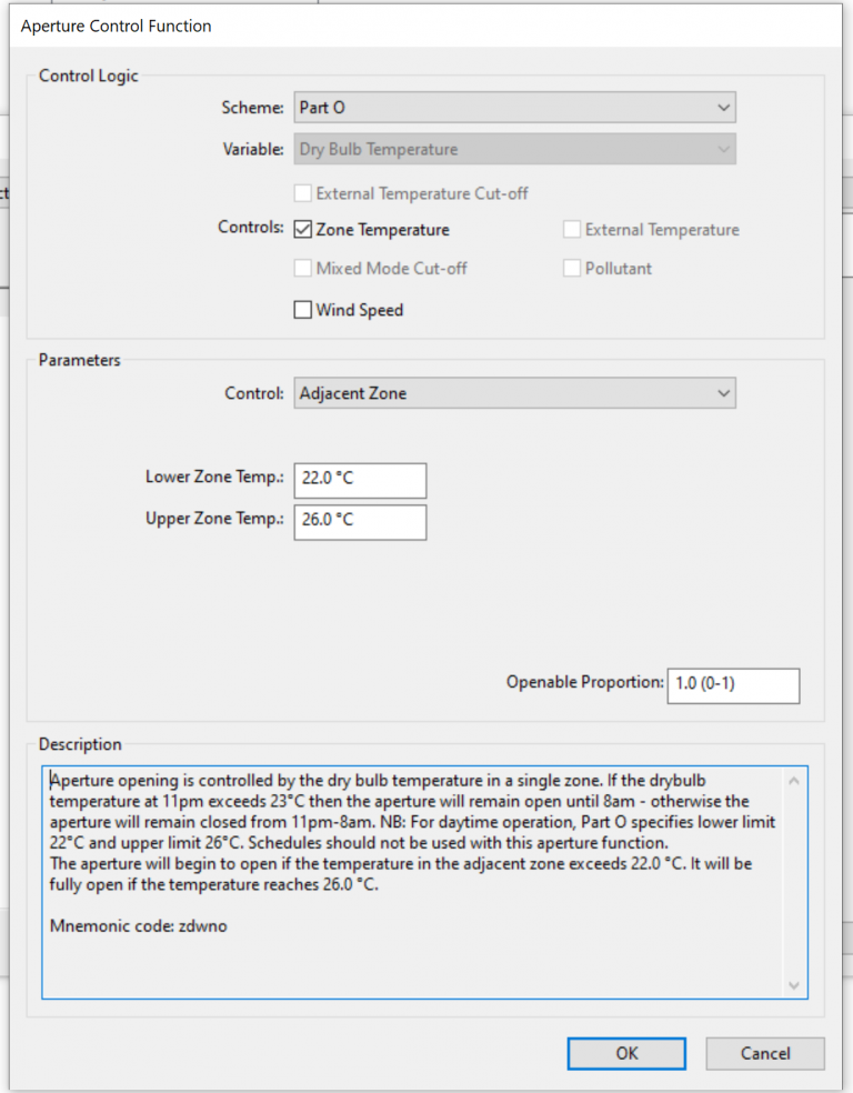
In Tas version 9.5.4 we have introduced a new aperture function specifically for Approved Document O.

Simply set up your models as you would for TM59 and apply the above aperture function to openings which are safe to open at night.

The day operation of the function will reflect the input settings, and at night the apertures will automatically stay open if the temperature exceeds 23°C at 11pm.

Then run through the TM59 wizard as normal.

Part O Aperture Function in Tas.

What else is new?

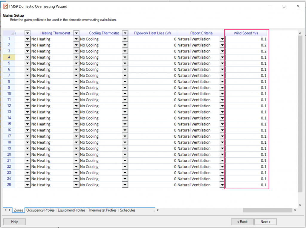
In addition to the new aperture function for part O, Tas v9.5.4 also allows you to model the effect of ceiling fans and other means of reliably generating air movement:

TM59 wizard screenshot showing wind speed column

Increased air movement can help reduce the temperature a person experiences when there are warm radiant surfaces present.

This functionality has also been added to our TM52 Adaptive Overheating report.

Where can I find more information about TM59 and Approved Document O?

In addition to the official TM59 document and the offical Approved Document O document, please see our TM59 documentation for more information about Approved Document O and TM59 in Tas.

Migrating from Hevacomp to Tas

Migrating from Hevacomp to Tas

Are you a Hevacomp user in need of a new tool for your building load and energy calculations? If so, in this post, we’ll look at how you can perform heat sizing and cooling sizing load calculations in Tas. 

You can also see an example heat sizing report and an example cooling sizing report from Tas. 

New Projects: Create the geometry

Creating new projects in Tas is a lot like Hevacomp. Start with the geometry, generate a building simulator file and provide constructions and weather details. 

You can create geometry by importing a DWG file and tracing around it. Label the spaces by assigning a zone, then export to the Building Simulator to assign constructions, weather & internal conditions. 

For existing projects, you can import IDF files from Hevacomp or use our gbXML import. 

New Projects: Select Weather & Assign Constructions

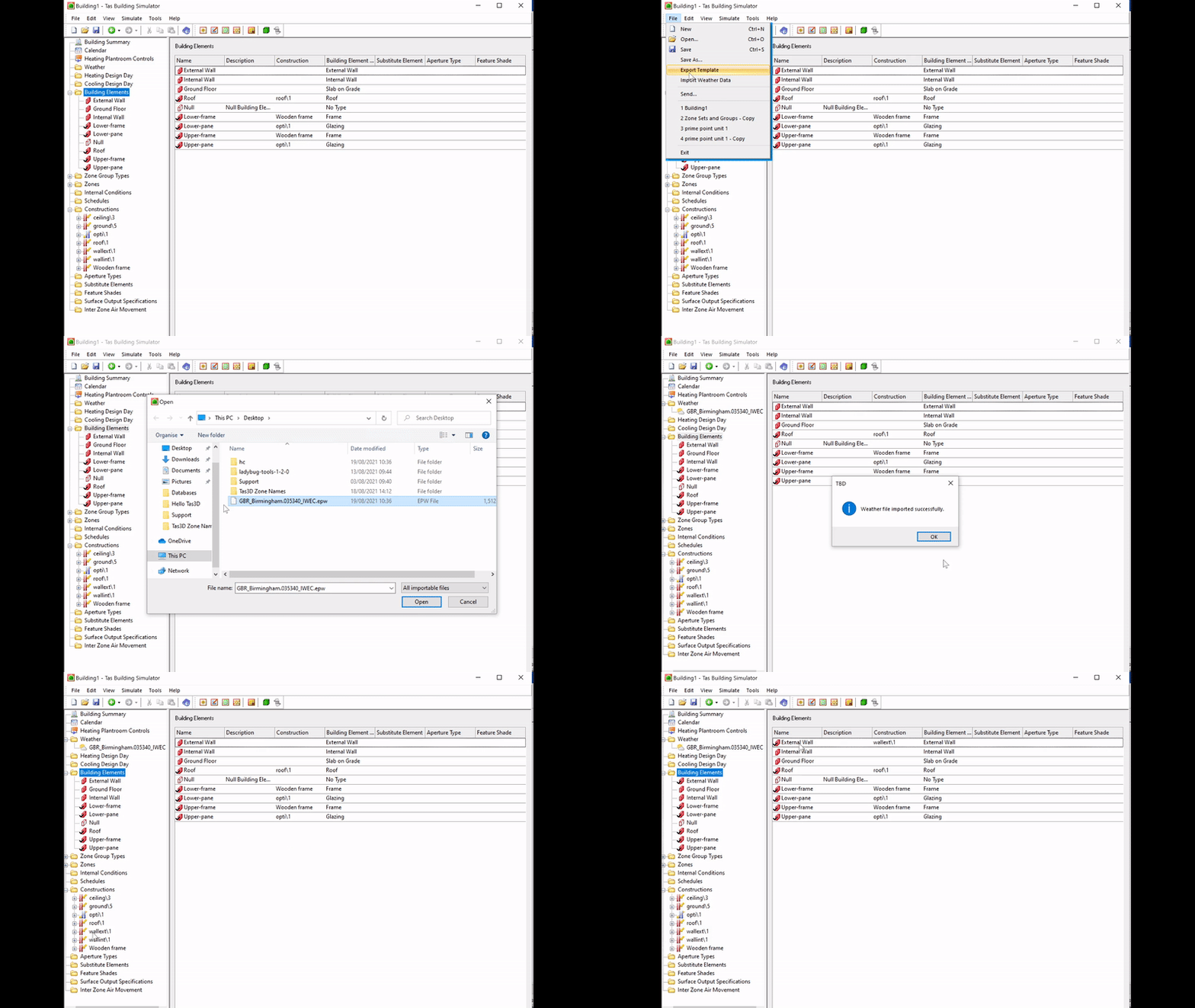
You can import an EPW weather file directly into the building simulator, use CIBSE weather or create your own weather file. 

You can assign constructions to your Building Simulator file from one of our databases bundled with the software, or you can create your own constructions by building up the material layers.

Calculating Loads using the Design Day Wizard

Once you’ve created a building simulator file with appropriate weather and constructions, you can launch the Design Day Wizard via: Tools > Design Day Wizard.

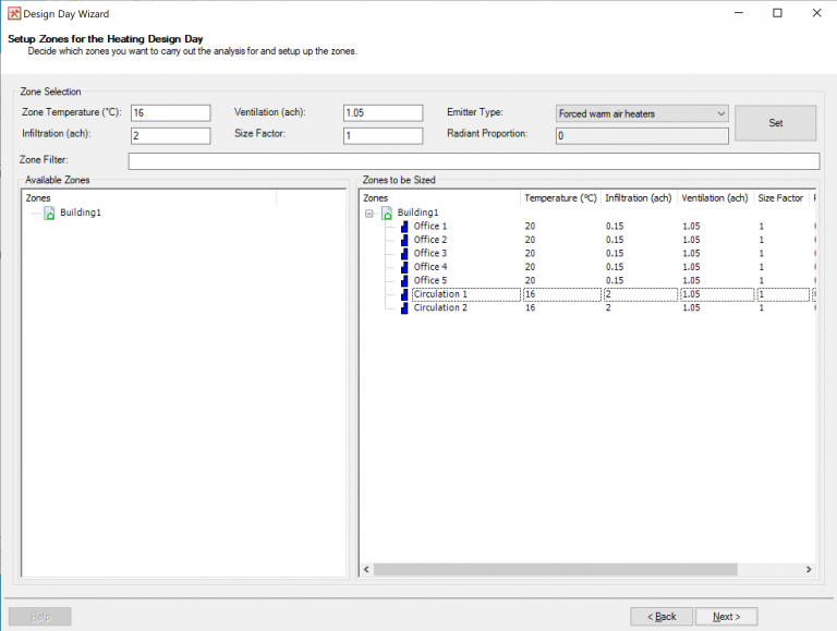
This wizard will guide you through performing heating & cooling load calculations. For heating loads, enter the heating setpoint and infiltration rate and the wizard will generate the heat loss report. 

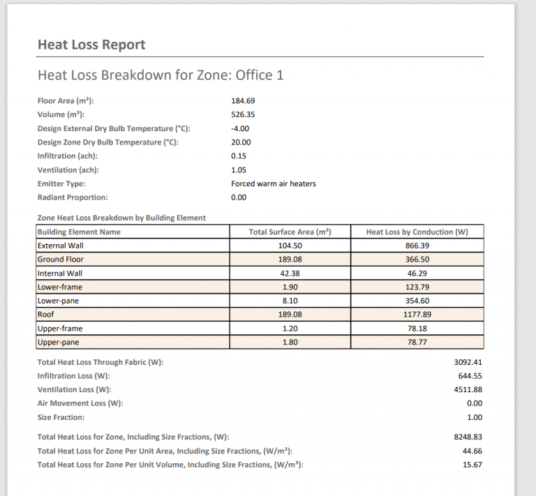
The heat loss report is generated for each of the zones selected in the wizard showing the breakdown through the building fabric. You can easily re-run the wizard to make amendments and generate a new report. 

Admittance Calculations & Pipe/Duct Sizing

For pipe & duct sizing, Tas integrates with MEPWorx, (formally Cymap). Data is transferred from your detailed HVAC simulation models. 

Importing Hevacomp files into Tas

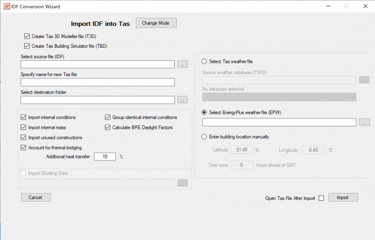
Tas can import both gbXML and IDF files; the best way to import existing Hevacomp projects into Tas is with our IDF import wizard:

Using the IDF Import wizard, you can automatically create a Tas3D file to perform daylight calculations on. The wizard will also create a building simulator file with internal gains, construction information and create a weather file for you either using an EPW or a native Tas TWD file.

You can find the IDF wizard in the Utilities folder of the Tas Manager. 

Improve Efficiency with Dynamic Simulation

So far we’ve examined how you can calculate heating and cooling loads using Tas using the steady state method. As Tas is a dynamic simulation package, you can also simulate a full year and determine peak loads that are more representative of the actual demand for heating and cooling, therefore preventing oversizing and undersizing, and leading to far more efficient building operation.

This can save energy, money and reduces the carbon footprint of the building. 

Ready to try it?

If you’re an existing Hevacomp user and wish to try Tas Engineering, you can download a free trial. To get started quickly, try using the IDF wizard to import an existing project of yours so you can explore the Design Day Wizard. If you have lots of users who would like a trial or have any specific questions, contact us. 

If you wish to create new projects in Tas, sign up for our free online e-trianing. 

Learn to Code with Tas and Excel Lesson 4- Tas3D Zone Writer pt 3

Learn to Code with Tas and Excel Lesson 4- Tas3D Zone Writer pt 3

In the last lesson, we modified our zone writer macro to:

  • Check for duplicate zone names
  • Check for existing zone groups and add zones to groups if they already exist

In this lesson, we’ll take a look at performance. So far, our macro works very well for adding a small number of zones to a model but as our model and the number of zones gets bigger, it can take a very long time to run!

Do I really need to worry about performance?

Usually, the time to start worrying about performance is when we try and use our macro and it takes a long time to run. After all, the whole point of writing these macros is to save time! 

Getting a feel for the difference between fast code and slow code is quite useful though, as it you’ll intuitively write fast code from the start and develop an intuition for how to keep things snappy. 

Lets time our macro

Lets modify our existing macro so we can time how long it takes to run. First, lets add a new subroutine called TimeAddZoneNames. We’ll use this function to call our existing function, AddZoneNames, and time how long it took to run:

				
					Sub TimeAddZoneNames()
    
    'Declare some variables to keep track of when we started timing and how much time has elapsed
    Dim StartTime As Double
    Dim SecondsElapsed As Double
    
    'Use the built in 'Timer' function to get the current number of seconds since midnight
    StartTime = Timer
    
    'Call our macro that adds zones to our model
    AddZoneNames
    
    'Call timer again, and calculate the difference in seconds
    SecondsElapsed = Round(Timer - StartTime, 2)
    
    'Display a message showing the time it took to run
    MsgBox "This code ran successfully in " & SecondsElapsed & " seconds", vbInformation
End Sub


We’ll also need to modify our AddZoneNames subroutine to remove the ‘finished’ messagebox at the end. 

Think about it

Why do we need to remove the finished message box from AddZoneNames?

Answer

If we didnt remove the message box, our timer would time how long it takes us to press OK to the Finished message box. We're interested in timing how long it takes to add zones to the 3D modeller file, not how quickly we can press Finished!

Last but not least, we’ll need to change the button we use to run our macro to call our TimeAddZoneNames subroutine:

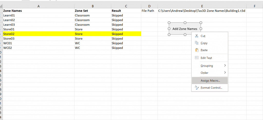
To do this, right click on the button and press Assign Macro. 

How long does it take to run?

Using the above modifications, i’ve timed how long it takes to run our macro when we’re adding a variable number of zones to the model. Results below. 

When we’re only adding 30 zones, the macro takes 3.5 seconds to run. Pretty good.

When we want to add 200 zones, it takes over a minute. Maybe that’s ok, we can usually spare a minute.

When we want to add 500 zones, it takes over 12 minutes!! This is not good. What if we make a mistake and need to re-run it? that’s almost half an hour of wasted time!

These times are from a fast 4GHz processor – take a moment to see how long it takes to add 200 zones on your machine and see how the times compare. 

Why does it take so long to run?

You might be wondering why this macro takes so long to run when computers can perform billions of calculations every second. Lets time how long a simple operation such as an addition takes:

				
					Sub addMillionTimes()
    Dim i As Long
    i = 0
    While i < 1000000
        i = i + 1
    Wend
End Sub


I timed calling this function, which adds 1 to a variable 1 million times, to see how long it would take to execute. Even with declaring the variable and assigning space for it in the computer RAM, this macro took 0.01 seconds to run!

Now lets compare it to a function which retrieves the building name in a file:

				
					Sub getBuildingNameMillionTimes(doc As TAS3D.T3DDocument)
    Dim i As Long
    Dim name As String
    i = 0
    While i < 1000000
        name = doc.Building.name
        i = i + 1
    Wend
End Sub


This subroutine takes a jaw dropping 46 minutes to run! Why? Because when we use a type library to control another application, the Windows operating system has to perform many security checks each time we call a function belonging to that library. Therefore, if we want to write fast macros, we need to reduce any unnecessary type library function calls.

In the case of our existing macro, every time we add a zone to the file we need to check every single zone in the file to see if it already exists. If we have 10 zones in the file and we want to add another, we have to check 10 zones before we can add a new one. A checking operation involves getting a reference to a Zone object then reading its name (3 operations). 

If we have 499 zones in our file, we have to check 499 zones names before we can add another one. 

But what if we could check each of the zone names once and remember the result, so that next time we want to add one we can save a lot of time? 

Dictionaries

Fortunately, we can use an object called a Dictionary in order to create a lookup table in the computers memory of zone names and zone references. 

Before we start adding zones to our file, we can read all the zones in the 3D modeller file once and add them to our lookup table. 

				
					Function CreateZoneDictionary(doc As TAS3D.T3DDocument) As Scripting.Dictionary
    Dim lookup As Dictionary
    Set lookup = New Scripting.Dictionary
    Dim curZone As TAS3D.Zone
     
     
    Dim curZoneIndex As Integer
    curZoneIndex = 0
    
    While Not doc.Building.GetZone(curZoneIndex) Is Nothing
        
        'Get a reference variable for the current zone
        Set curZone = doc.Building.GetZone(curZoneIndex)
        
        lookup.Add curZone.name, curZone
            
        
        'incremenet the zone index so we look at the next one in the file when the loop repeats
        curZoneIndex = curZoneIndex + 1
    Wend
    
    Set CreateZoneDictionary = lookup
    
End Function


Note that in order to use Dictionaries, you need to reference the Microsoft Scripting Runtime via Tools > References.

This function creates a dictionary on line 3, and then iterates over every zone in the file. On line 15, it stores the zone name as the dictionary key and a reference to the zone as the value in the dictionary. 

We can therefore use the dictionary to very quickly retrieve a reference to a zone using its name. Using this dictionary, we can re-write our ZoneExists function:

				
					Function ZoneExists(name As String, lookup As Scripting.Dictionary) As Boolean
    
  ZoneExists = lookup.Exists(name)
   
End Function


Looking up a value in a dictionary based on its key is extremely fast, as no type library function calls are required. 

Putting it all together

The complete macro, with the changes highlighted, can be seen below. I have also created a dictionary for zoneSets in order to speed up checking of zone sets exist already, and adding zones to them. 

				
					Sub TimeAddZoneNames()
    Dim StartTime As Double
    Dim SecondsElapsed As Double
    
    StartTime = Timer
    
    AddZoneNames

    SecondsElapsed = Round(Timer - StartTime, 2)
    
    MsgBox "This code ran successfully in " & SecondsElapsed & " seconds", vbInformation
End Sub


Sub AddZoneNames()
    'Read the file path from the spreadsheet
    Dim filePath As String
    filePath = Cells(1, 5)

    'Open the 3D modeller
    Dim t3dApp As TAS3D.T3DDocument
    Set t3dApp = New TAS3D.T3DDocument

    'Declare a variable for checking if operations were successful
    Dim ok As Boolean

    'Try to open the existing file
    ok = t3dApp.Open(filePath)

    'Check if it did open successfully
    If Not ok Then
        MsgBox "Couldnt open the file; is it in use?"
        Exit Sub
    End If
    

    'Define our loop variables
    Dim rowIndex As Integer
    Dim zoneName As String
    Dim zoneSetName As String
    Dim newZone As TAS3D.Zone
    Dim zoneSet As TAS3D.zoneSet

    'Set the starting rowIndex
    rowIndex = 2
    
    'lookups
    Dim zoneLookup As Dictionary
    Dim zoneSetLookup As Dictionary
    Set zoneLookup = CreateZoneDictionary(t3dApp)
    Set zoneSetLookup = CreateZoneSetDictionary(t3dApp)
    

    'Check each zone name cell to see if it contains something
    While Not IsEmpty(Cells(rowIndex, 1))

        'Read the zone name from excel
        zoneName = Cells(rowIndex, 1)
        
        'Read the zone set name from excel
        zoneSetName = Cells(rowIndex, 2)

        'Check that the zone name isnt already in use
        If ZoneExists(zoneName, zoneLookup) Then
            Cells(rowIndex, 3) = "Skipped"
        Else
            'Check to see if there is a zone set already in the file with the right name
            Set zoneSet = GetZoneSet(zoneSetName, zoneSetLookup)
            
            'If it doesnt exist, make a zone set wtih that name
            If zoneSet Is Nothing Then
                Set zoneSet = t3dApp.Building.AddZoneSet(zoneSetName, "", 0)
                
                'Add it to the dictionary
                zoneSetLookup.Add zoneSetName, zoneSet
            End If
            
            'Add a zone to the zone set
            Set newZone = zoneSet.AddZone()
            
            'Change the name of the zone we just added
            newZone.name = zoneName
            
            'Add it to the dictionary
            zoneLookup.Add zoneName, newZone
            
            'Note the addition was a success
            Cells(rowIndex, 3) = "added"
            
        End If


        'Increment the row index (so we read the next cell down)
        rowIndex = rowIndex + 1

    Wend

    'Save the file and check the save was successful
    ok = t3dApp.Save(filePath)

    If Not ok Then
        MsgBox "Couldn't save the file!"
        Exit Sub
    End If

    'Close the file
    t3dApp.Close

    'Close the 3D modeller
    Set t3dAppp = Nothing


End Sub

Function CreateZoneDictionary(doc As TAS3D.T3DDocument) As Scripting.Dictionary
    Dim lookup As Dictionary
    Set lookup = New Scripting.Dictionary
    Dim curZone As TAS3D.Zone
     
     
    Dim curZoneIndex As Integer
    curZoneIndex = 0
    
    While Not doc.Building.GetZone(curZoneIndex) Is Nothing
        
        'Get a reference variable for the current zone
        Set curZone = doc.Building.GetZone(curZoneIndex)
        
        'Add the zone to the dictionary, using its name as the key
        lookup.Add curZone.name, curZone
            
        
        'incremenet the zone index so we look at the next one in the file when the loop repeats
        curZoneIndex = curZoneIndex + 1
    Wend
    
    Set CreateZoneDictionary = lookup
    
End Function

Function CreateZoneSetDictionary(doc As TAS3D.T3DDocument) As Scripting.Dictionary
    Dim lookup As Dictionary
    Set lookup = New Scripting.Dictionary
    Dim curSet As TAS3D.zoneSet
     
     
    Dim curZoneSetIndex As Integer
    curZoneSetIndex = 0
    
    While Not doc.Building.GetZone(curZoneSetIndex) Is Nothing
        
        'Get a reference variable for the current zone
        Set curSet = doc.Building.GetZoneSet(curZoneIndex)
        
        'Add the current zone set to the dictionary, using its name as the key
        lookup.Add curSet.name, curSet
            
        'incremenet the zone index so we look at the next one in the file when the loop repeats
        curZoneSetIndex = curZoneSetIndex + 1
    Wend
    
    Set CreateZoneSetDictionary = lookup
    
End Function

Function ZoneExists(name As String, lookup As Scripting.Dictionary) As Boolean
    
  ZoneExists = lookup.Exists(name)
    
End Function

Function GetZoneSet(name As String, lookup As Scripting.Dictionary) As TAS3D.zoneSet
    
    If lookup.Exists(name) Then
    
        Set GetZoneSet = lookup(name)
        
    Else
    
        Set GetZoneSet = Nothing
        
    End If
  
End Function


As we have already discussed how dictionaries work, we wont go through this macro line by line – hopefully the comments will be enough to explain what’s going on, along with your experience from the lessons so far. 

How much time did we save?

The amount of time we saved by using dictionaries might shock you. 

To add 1,000 new zones using dictionaries took only 2.16 seconds. With the old version, it took over 12 minutes to add half that number!

Details: Dictionaries

Dictionaries are common in most programming languages, but sometimes they go by other names such as ‘Hash Maps’. A dictionary is an object that can store a number of pairs of items. These pairs consist of a Key and a Value.

The Key can be of any type, as can the Value. 

Each key in a dictionary must be unique — that is, you cant have the same key in there multiple times!

If you’re still unsure what a dictionary is, you can think of it as a kind of lookup table. Imagine you had a table of council tax bands and the prices you’d pay for each band:

Band Price
A £20,000
B £30,000
C £43,000
D £51,000

Here, the band is the key and the price is the value. If you wanted to find out the price for being in a band, you’d look it up in the table. 

Dictionaries have functions that allow you to:

  • See if there is an entry in a dictionary for a key already (dictionary.exists)
  • Add items (dictionary.add)
  • Remove items (dictionary.remove)

For more information about dictionaries, see the Excel Macro Mastery topic on the subject. 

Next Lesson

In this lesson we’ve learned something very important – that we should try to call certain type libraries functions as infrequently as possible in order to write fast macros. We’ve also looked at one way in which we can achieve this – by calling these functions once and storing the result to use later, so we don’t have to check again.

In the next lesson, we’ll move on from our zone writer macro and write one to perform some daylight calculations in the 3D modeller. We’ll also learn how to read the lux values for each point and write them to our spreadsheet.